Allrecipes.com Hall of Fame analysis
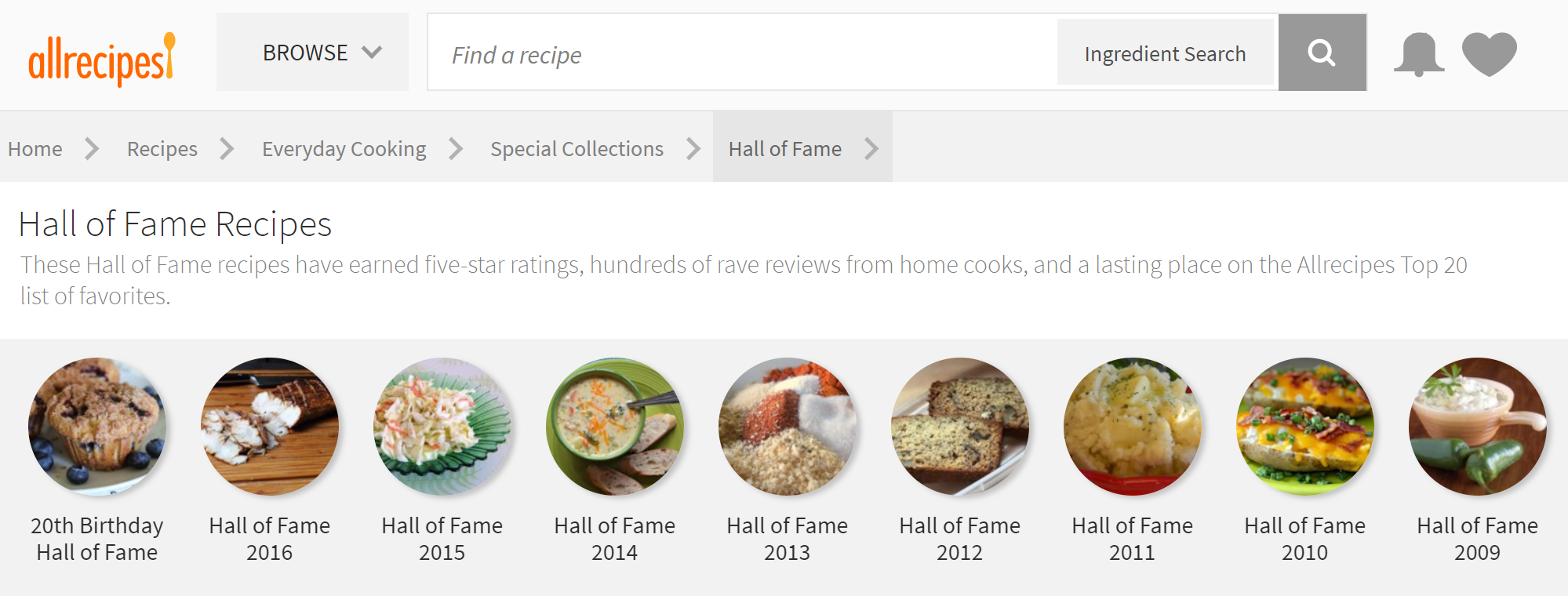
This post will explore the recipes included in Allrecipes.com’s Hall of Fame collection, a yearly compilation of 20 recipes that were most popular with the site’s users. It is also the first project I have done using R.
Data Acquisition
I used Selenium through Python to iterate over each yearly Hall of Fame collection, acquiring the list of recipes. Each recipe was then scraped.
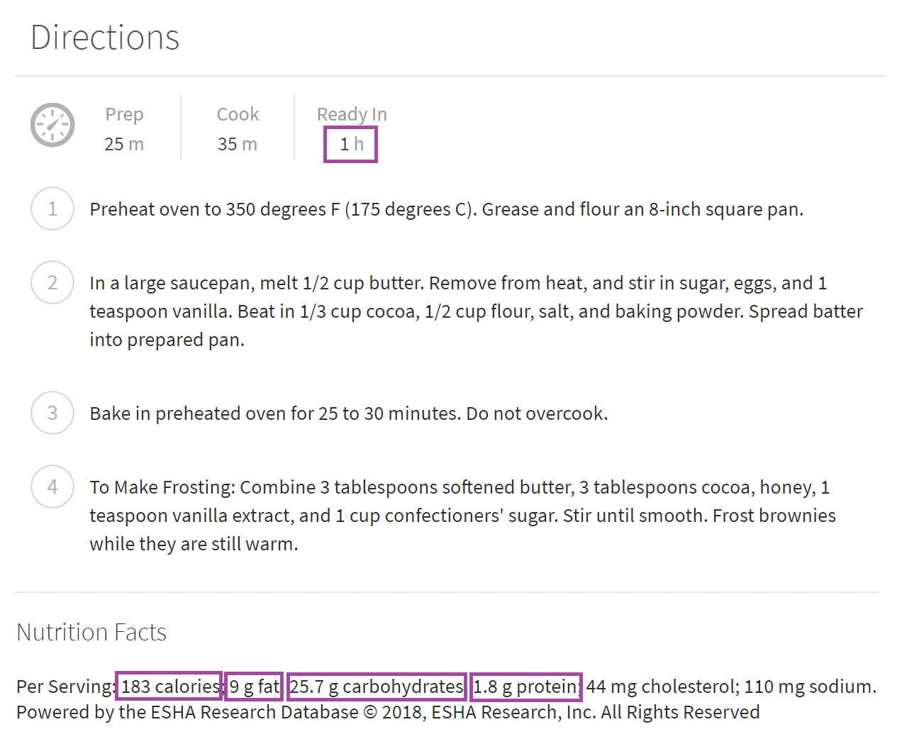
- I picked out the basics, such as the title of the recipe and social metrics, like the number of photos associated with the recipe, the number of people who indicated they had made it, and the number of reviews of the recipe.

- I also found the ingredients in each recipe, and the number of servings the recipe makes.
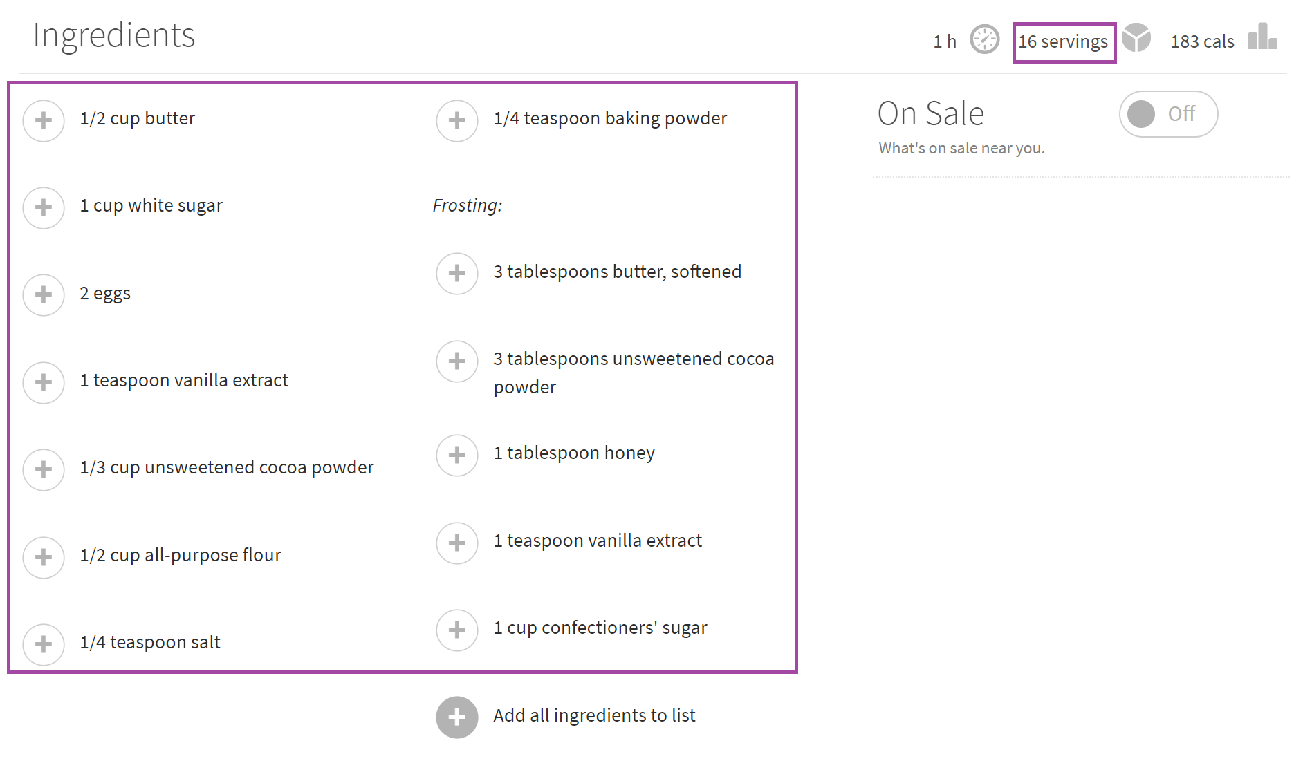
- I found the nutrition breakdown for each recipe - calories, carbs, fat, and protein (all by serving), as well as the amount of time the recipe takes to complete.
Please note that the data used in this analysis is not mine, and so I have not hosted it online. However, the code I used to access Allrecipes.com’s public-facing data can be found in my Git repository and should run happily as long as Allrecipes.com does not change their site format.
Import data
Moving to R, the first step is to read in the data (removing the first column, an index courtesy of pandas).
df = read.csv('allrecipes.csv', stringsAsFactors=FALSE)[,-1]

head(df, n=2L)

##                         year                       title  ratings madeit
## 1 20th-birthday-hall-of-fame Best Chocolate Chip Cookies 4.603897    27K
## 2 20th-birthday-hall-of-fame     Homemade Mac and Cheese 4.101205     7K
## 3 20th-birthday-hall-of-fame Good Old Fashioned Pancakes 4.589163    20K
##   reviews photos
## 1    9429     2K
## 2    1592    328
## 3    9611    851
##                                                                                                                                 submitter_description
## 1                                                                                                                       "Crisp edges, chewy middles."
## 2                                            "This is a nice rich mac and cheese. Serve with a salad for a great meatless dinner. Hope you enjoy it."
## 3 "This is a great recipe that I found in my Grandma's recipe book. Judging from the weathered look of this recipe card, this was a family favorite."
##                                                                                                                                                                                                                                                                             ingredients
## 1 ['1 cup butter, softened', '1 cup white sugar', '1 cup packed brown sugar', '2 eggs', '2 teaspoons vanilla extract', '3 cups all-purpose flour', '1 teaspoon baking soda', '2 teaspoons hot water', '1/2 teaspoon salt', '2 cups semisweet chocolate chips', '1 cup chopped walnuts']
## 2                             ['8 ounces uncooked elbow macaroni', '2 cups shredded sharp Cheddar cheese', '1/2 cup grated Parmesan cheese', '3 cups milk', '1/4 cup butter', '2 1/2 tablespoons all-purpose flour', '2 tablespoons butter', '1/2 cup bread crumbs', '1 pinch paprika']
## 3                                                                                                          ['1 1/2 cups all-purpose flour', '3 1/2 teaspoons baking powder', '1 teaspoon salt', '1 tablespoon white sugar', '1 1/4 cups milk', '1 egg', '3 tablespoons butter, melted']
##   readyin servings calories  fat carbohydrate protein
## 1     1 h       24      298 15.6         38.8     3.6
## 2    50 m        4      858 48.7         66.7    37.7
## 3    20 m        8      158  5.9         21.7     4.5
Sanity Checks
To make sure the data was scraped properly, I’ll perform a few checks first.
Checking for scale
cat("Number of years in sample:", length(unique(df$year)), '\n')

## Number of years in sample: 21

cat("Number of unique recipes in sample:", length(unique(df$title)), '\n')

## Number of unique recipes in sample: 290

cat("Number of recipes featured in multiple years:",
    length(unique((df %>% group_by(title) %>% filter(n()>1))$title)))

## Number of recipes featured in multiple years: 59
All of these seem logical with the amount of data I thought I scraped.
Imputation
Next, let’s check for NA values, where the scraper wasn’t able to bring the data in.
for (col in colnames(df)) {
  cat("Number of missing values in", col, ":", sum(is.na(df[[col]])), '\n')
}

## Number of missing values in year : 0
## Number of missing values in title : 0
## Number of missing values in ratings : 0
## Number of missing values in madeit : 0
## Number of missing values in reviews : 0
## Number of missing values in photos : 0
## Number of missing values in submitter_description : 0
## Number of missing values in ingredients : 0
## Number of missing values in readyin : 0
## Number of missing values in servings : 0
## Number of missing values in calories : 2
## Number of missing values in fat : 2
## Number of missing values in carbohydrate : 2
## Number of missing values in protein : 2
Seems to be a pretty complete dataset. Let’s further investigate the 2 missing rows for the nutrition information breakdown, which are possibly the same 2 recipes for each missing column (calories, fat, carbohydrate, protein).
df[is.na(df$calories),c(1,2,11,12,13,14)]

##     year          title calories fat carbohydrate protein
## 150 2010   Turkey Brine       NA  NA           NA      NA
## 153 2010 Perfect Turkey       NA  NA           NA      NA
Sure enough, the missing values hail from the same two recipes. As this is a mainly descriptive analysis, I’ll simply fill these two recipe’s missing values with the median, to avoid skewing any visuals.
for (col in colnames(df)[seq(11,14)]) {
  df[[col]][is.na(df[[col]])] = median(df[[col]], na.rm=TRUE)
  cat("New number of missing values in", col, ":", sum(is.na(df[[col]])), '\n')
}

## New number of missing values in calories : 0
## New number of missing values in fat : 0
## New number of missing values in carbohydrate : 0
## New number of missing values in protein : 0
Data Munging
Let’s check each column’s formatting, and perform any necessary transformations to get numerical data wherever possible. First, the ‘readyin’ column, since the format is mixed minutes/hours.
cat(paste(unique(df$readyin)[1:20], collapse=';\n'))

## 1 h;
## 50 m;
## 20 m;
## 1 h 20 m;
## 7 h 10 m;
## 25 m;
## 45 m;
## 8 h 10 m;
## 30 m;
## 1 h 10 m;
## 3 h 15 m;
## 12 h 20 m;
## 2 h 31 m;
## 40 m;
## 1 h 40 m;
## 2 h;
## 6 h 10 m;
## 35 m;
## 1 h 15 m;
## 15 m
For uniformity, I’ll combine all these times into one unit, minutes.
clean_minutes = function(text) {
  time = 0
  if (grepl(' d', text, fixed=TRUE)) {
time = time + as.numeric(substr(text, 1, regexpr(" d", text)[1]-1))*24*60
text = substr(text, regexpr(" d", text)[1]+2, nchar(text))
  }
  if (grepl(' h', text, fixed=TRUE)) {
time = time + as.numeric(substr(text, 1, regexpr(" h", text)[1]-1))*60
text = substr(text, regexpr(" h", text)[1]+2, nchar(text))
  }
  if (grepl(' m', text, fixed=TRUE)) {
time = time + as.numeric(substr(text, 1, regexpr(" m", text)[1]-1))
text = substr(text, regexpr(" m", text)[1]+2, nchar(text))
  }
  return(time)
}

df$readyin = sapply(df$readyin, clean_minutes)
summary(df$readyin)

## Min.  1st Qu.   Median Mean  3rd Qu. Max.
## 0.00 34.2560.00   157.63   100.00 13000.00
Also note that the 2017 Hall of Fame was listed as the ‘20th Birthday Hall of Fame’, so let’s take care of that while we convert the ‘year’ column to integers.
df$year[df$year=="20th-birthday-hall-of-fame"] = 2017
df$year = suppressWarnings(as.numeric(df$year))
unique(df$year)

##  [1] 2017 2016 2015 2014 2013 2012 2011 2010 2009 2008 2007 2006 2005 2004
## [15] 2003 2002 2001 2000 1999 1998 1997
Sure enough, we know have recipes for each year from 1997 through 2017.
Let’s also clean up the social metrics (number of people who ‘made it’ and number of photos related to the recipe), since the site formats the numbers imprecisely.
clean_numbers_social = function(text) {
  if (grepl('K', text, fixed=TRUE)) {
    return(as.numeric(substr(text, 1, nchar(text)-1))*1000)
  }
  else {
    return(as.numeric(text))
  }
}
df$madeit = sapply(df$madeit, clean_numbers_social)
summary(df$madeit)

##Min. 1st Qu.  MedianMean 3rd Qu.Max.
##15.0   609.2  2000.0  4722.4  8000.0 27000.0

df$photos = sapply(df$photos, clean_numbers_social)
summary(df$photos)

## Min. 1st Qu. Median Mean 3rd Qu.  Max.
## 1.0   32.0   107.5 301.7  422.0  2000.0
Exploratory Analysis
library(corrplot)

cor_matrix = cor(df[,c(4,5,6,9,10,11,12,13,14)])

corrplot(cor_matrix, type = "upper", order = "hclust",
         tl.col = "black", tl.srt = 45,
         col=colorRampPalette(c("#07337a", "#7483f9", "#55c184", "#eef975"))(100))
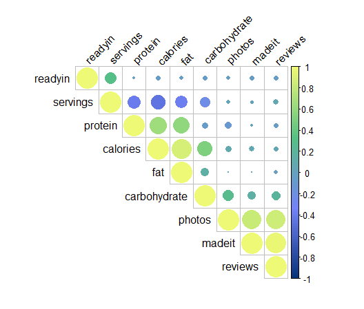
We can see there are significant positive correlations between the social metrics, such as number of photos, number of reviews, and the number of people who indicated they ‘made it’ for each recipe.
We can also see negative correlation between the number of servings and the protein, calories, fat, and carohydrate counts. This is rather interesting, as the nutrition measures are per-serving, perhaps because the ‘serving size’ is subjective information, provided by the recipe author, and so not standardized across the website. With this story, it is clear that some authors prefer smaller serving sizes (low calorie/fat/etc founts), but bake the same quantity of food in a larger number of portions (high serving size), while other authors take the reverse approach, preparing the same quantity of food divided into fewer portions, with higher calorie/fat/etc counts per-serving.
library(ggplot2)
library(ggthemes)

## Warning: package 'ggthemes' was built under R version 3.4.3

ts = df %>% select(servings, calories, fat, protein, carbohydrate, year) %>% group_by(year) %>%  summarise_all(funs(mean))

ggplot(ts, aes(year, calories)) +
  geom_line(aes(y=calories), col="#07337a") +
  coord_cartesian(ylim = c(0, 425)) +
  theme_bw() +
  ggtitle('Average Calories per Serving, by Year') +
  theme(
plot.title = element_text(hjust = 0.5)
  )
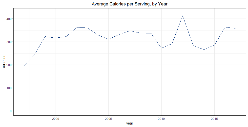
There is perhaps a slight increasing trend in the number of calories per serving, though the majority of this increase happens in the first few years (1997-1999) and the rest of the deviations seem to be somewhat random.
ggplot(ts, aes(year, servings)) +
  geom_line(aes(y=servings), col="#07337a") +
  coord_cartesian(ylim = c(0, 50)) +
  theme_bw() +
  ggtitle('Average Number of Servings per Recipe, by Year') +
  theme(
plot.title = element_text(hjust = 0.5)
  )
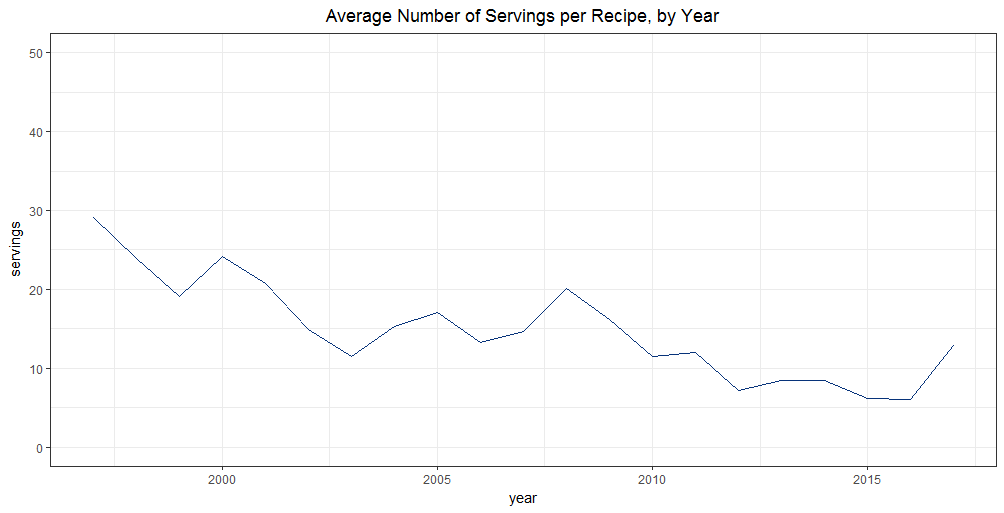
We can see an obvious downward trend in the number of servings per recipe, perhaps due to an increased interest in cooking for smaller families or 2-person households.
ggplot(data = ts, aes(x = year)) +
  geom_line(aes(y = fat, colour = "Fat")) +
  geom_line(aes(y = protein, colour = "Protein")) +
  geom_line(aes(y = carbohydrate, colour = "Carbohydrate")) +
  scale_colour_manual("",
  breaks = c("Carbohydrate", "Fat", "Protein"),
  values = c("Fat"="#07337a", "Protein"="#7483f9",
 "Carbohydrate"="#55c184")) +
theme_bw() +
  labs(title="Nutrition Break-Down, by Year", x="Year", y="Grams")+
  coord_cartesian(ylim = c(0, 50)) +
  theme(
plot.title = element_text(hjust = 0.5)
  )
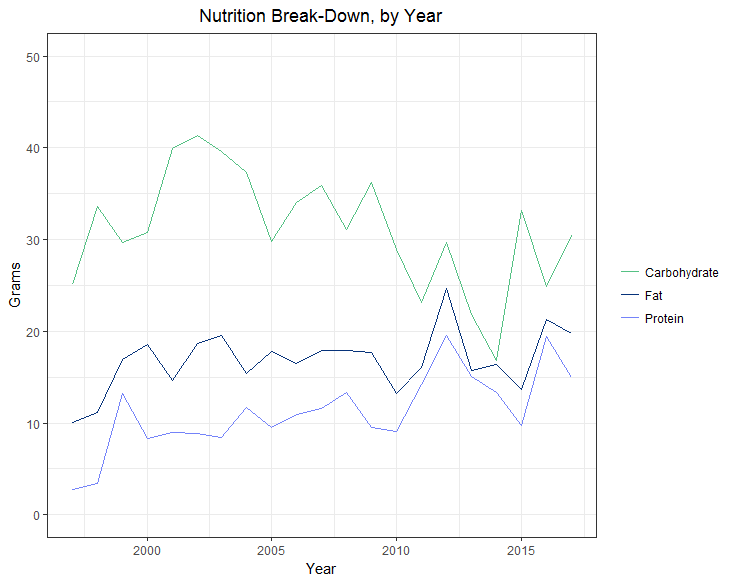
Here, we can clearly see that recipes have gotten healthier over time (as measured by the higher protein and fat content, and lower carbohydrate content). This is probably due to the increased interest in health over the past few years, with dietary movements like organic, gluten-free, and raw gaining support, and the change in dietary recommendations (healthy fat is now highly recommended, where before all fat was treated the same, to be avoided).
Text Examination
First, let’s see if there’s any pattern in the titles, like ‘easy’ or ‘best’ showing up frequently.
For cleanliness, since some of the titles contain roman numerals, like ‘Alfedo Sauce IV’, I’ll clean those from the ends of the strings, then lowercase all the titles, and move the text into a corpus.
library(wordcloud)
library(tm)

titles = tm_map(Corpus(VectorSource(gsub(" [IXV]+$", "", df$title, perl=TRUE))), content_transformer(tolower))
cat(titles[seq(1:10)]$content, sep="\n")

## best chocolate chip cookies
## homemade mac and cheese
## good old fashioned pancakes
## banana banana bread
## slow cooker pulled pork
## easy sugar cookies
## buffalo chicken dip
## awesome slow cooker pot roast
## basic crepes
## chicken pot pie
Next, let’s count some words to see what our most dramatic components are, and build a wordcloud. I’ll also remove stopwords, to prevent words like ‘and’ appearing frequently.
titles = tm_map(titles, removeWords, stopwords("english"))
doc_term_mat = as.matrix(TermDocumentMatrix(titles))
doc_term_mat = sort(rowSums(doc_term_mat), decreasing=TRUE)
d = data.frame(word = names(doc_term_mat), freq=doc_term_mat)

set.seed(5)
wordcloud(words = d$word, freq = d$freq, min.freq = 6,
		  random.order = FALSE, random.color = FALSE,
		  rot.per=0.3, colors=brewer.pal(11, "Spectral"))
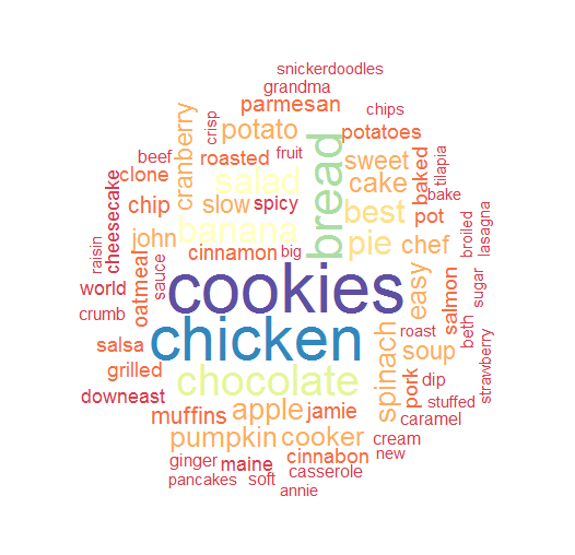
Here, we can clearly see that cookie recipes are more dominant than any other type, followed by chicken, then bread and chocolate.
Let’s perform a similar analysis on the submitter descriptions.
sub_des = tm_map(Corpus(VectorSource(gsub(" [IXV]+$", "", df$submitter_description, perl=TRUE))), content_transformer(tolower))
cat(sub_des[seq(1:10)]$content, sep="\n")

## "crisp edges, chewy middles."
## "this is a nice rich mac and cheese. serve with a salad for a great meatless dinner. hope you enjoy it."
## "this is a great recipe that i found in my grandma's recipe book. judging from the weathered look of this recipe card, this was a family favorite."
## "why compromise the banana flavor? this banana bread is moist and delicious with loads of banana flavor! friends and family love my recipe and say it's by far the best! it's wonderful toasted!! enjoy!"
## "pork simmered in root beer makes all the difference. topped with your favorite bbq sauce, it's sure to bring rave reviews."
## "quick and easy sugar cookies! they are really good, plain or with candies in them. my friend uses chocolate mints on top, and they're great!"
## "this tangy, creamy dip tastes just like buffalo chicken wings. it's best served hot with crackers and celery sticks. everyone loves the results!"
## "this is a very easy recipe for a delicious pot roast. it makes its own gravy. it's designed especially for the working person who does not have time to cook all day, but it tastes like you did. you'll want the cut to be between 5 and 6 pounds."
## "here is a simple but delicious crepe batter which can be made in minutes. it's made from ingredients that everyone has on hand."
## "a delicious chicken pie made from scratch with carrots, peas and celery."

sub_des = tm_map(sub_des, removeWords, stopwords("english"))
doc_term_mat = as.matrix(TermDocumentMatrix(sub_des))
doc_term_mat = sort(rowSums(doc_term_mat), decreasing=TRUE)
d = data.frame(word = names(doc_term_mat), freq=doc_term_mat)

wordcloud(words = d$word, freq = d$freq, min.freq = 15,
		  random.order = FALSE, random.color = FALSE,
		  rot.per=0.3, colors=colorRampPalette(c("#07337a", "#55c184", "#eef975"))(7))
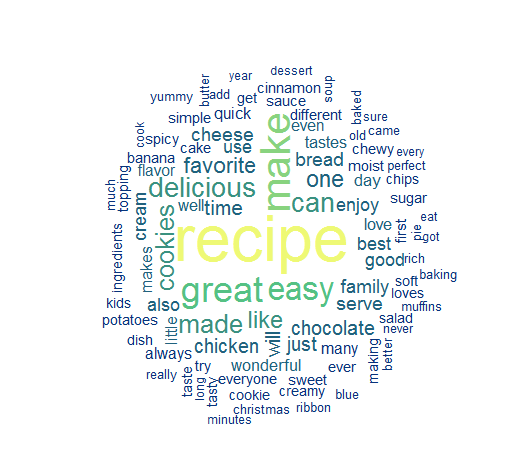
Apparently, the most generic submitter description would be “this is a great recipe, very easy to make, and delicious”. Also there’s a very clear split here between the highly frequent words (recipe, make, great), and the remaining words.
Code
The data scraping was with Python 3.5.1 and Selenium 3.6.0, using Chromedriver 2.35 for Windows.
Analysis was completed in RStudio using R 3.4.1, requiring on dplyr, ggplot2, corrplot, ggthemes, wordcloud, and tm.
Code for the scraper, analysis and visualizations can be found in my Example Projects Repository.