Targeting Wake County restaurants for better sanitation

Concerning Predictive Modeling, using Python on 2019/07/22

business case text

Using restaurant data to target “at-risk” restaurants for a mailing campaign with the goal of encouraging better practices in advance of their next inspection.

• Background
• Scenario
• Dataset
  • Cleaning
  • Exploration
• Making predictions
  • Approach
  • Feature engineering
  • Modeling
    • Balance classes
    • Separate input from output
    • Make/evaluate a random predictions
    • GridSearch for decision tree
    • GridSearch for bagging
    • GridSearch for boosting
    • GridSearch for random forest
  • Simulating the mailer
• Code

Background

Wake County provides open data for the public to analyze, including data on restaurant inspections. I’ve been meaning to use an open dataset for a while, and decided to start by inventing a prediction problem that would leverage their open data about restaurants and restaurant inspections in Wake County.

Scenario

At the end of 2018, the Wake County health department decides to implement a mailing campaign to increase awareness of food handling best practices, with the goal of decreasing the number of “at-risk” restaurants (those receiving an inspection score < 93).

Wake County can only send 500 mailers, and wants to use data science to successfully target as many “at-risk” restaurants in advance of their inspection as possible.

Dataset

We have 3 tables to work with, courtesy of Wake County Open Data:

• Restaurants
  Restaurants gives details on each restaurant location, such as NAME, PHONENUMBER, and RESTAURANTOPENDATE.
• Inspections
  Inspections gives details on each restaurant inspection. Most restaurants have multiple entries in inspections, including information like INSPECTDATE, INSPECTOR, and SCORE.
• Violations
  Violations details the violations detected in each restaurant inspection. Most inspections have multiple entries in violations, including information like CATEGORY, SEVERITY, and COMMENTS.

All datasets were pulled on 7/3/19.

Cleaning

Our first task is inspecting the datasets and tidying them up a bit.

rest = pd.read_csv('./data/Restaurants_in_Wake_County.csv', index_col=['OBJECTID'],
                  parse_dates=['RESTAURANTOPENDATE'], infer_datetime_format=True)

insp = pd.read_csv('./data/Food_Inspections.csv', index_col=['OBJECTID'],
                  parse_dates=['DATE_'], infer_datetime_format=True)

viol = pd.read_csv('./data/Food_Inspection_Violations.csv',
                  parse_dates=['INSPECTDATE'], infer_datetime_format=True, low_memory=False)

Looking at restaurants:

HSISID	NAME	CITY	POSTALCODE	PHONENUMBER	RESTAURANTOPENDATE	FACILITYTYPE	PERMITID
2001	4092030273	RARE EARTH FARMS (WCID #512)	RALEIGH	27606	(919) 349-6080	2015-01-16 00:00:00+00:00	Mobile Food Units	18359
2002	4092015000	GRACE Christian School Kitchen	RALEIGH	27606	(919) 783-6618	2007-11-06 00:00:00+00:00	Restaurant	3377

The CITY field is not standardized - we’ll fix it by turning all lowercase, and replacing hyphens with a space.

rest['CITY'] = rest['CITY'].str.lower().str.replace('-', ' ')

For simplicity, we’ll lump any CITY that contains less than 10 restaurants into an other category. Rows with missing CITY will also be lumped into other.

rest.loc[rest['CITY'].isin(rest['CITY'].value_counts()[rest['CITY'].value_counts()<10].index),
        'CITY'] = 'other'
rest['CITY'].fillna('other', inplace=True)

POSTALCODE isn’t standardized either - abbreviate to 5 digit format and treat as integer.

rest['POSTALCODE'] = rest['POSTALCODE'].apply(lambda st:int(st[:5]))

NAME is generally messy, as most freeform text fields are - in an effort to standardize, we’ll remove odd characters and lowercase.

from re import findall
rest['NAME'] = rest['NAME'].str.lower().str.replace('`', "'").apply(lambda x:' '.join(findall(r"([a-z'-]+)(?=\s|$)", x)))

Looking at inspections:

OBJECTID	HSISID	SCORE	INSPECTDATE	DESCRIPTION	TYPE	INSPECTOR	PERMITID
1001	4092015443	96.0	2015-03-24 00:00:00+00:00	NaN	Inspection	Caroline Suggs	4768
1002	4092015443	94.0	2015-09-25 00:00:00+00:00	Follow-Up: 10/05/2015	Inspection	Jennifer Edwards	4768

Interestingly, only about 97% of the rows in inspections can be connected to restaurants, and we need all the data for modeling, so we’ll only retain those that can be linked back to the other tables.

insp = insp[insp['HSISID'].isin(rest['HSISID'])]

We’re not going to use violations beyond a measure of how many violations each inspection found, so the majority of the columns are irrelevant. However, we will perform the same filter as we used on inspections, so that all violations can be connected to restaurants, using inspections as a crosswalk.

viol = viol.drop('HSISID', axis=1).join(insp.set_index('PERMITID')['HSISID'].drop_duplicates(),
         on='PERMITID', how='inner')

Exploration

Wake County is growing in population, and new restaurants are being opened each month. This means that the Wake County health department is performing more inspections each month. 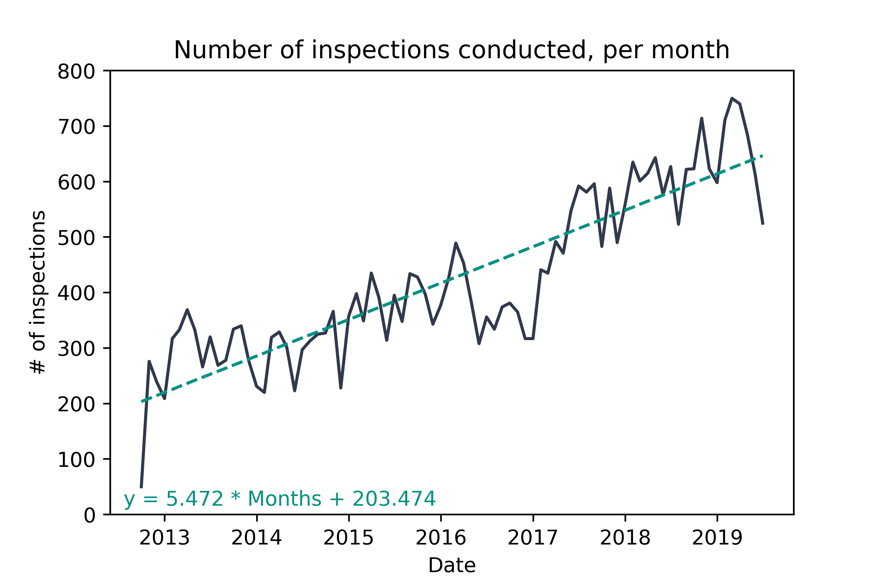Interestingly, we see that each inspection is detecting fewer inspections over time - whether this is due to an actual improvement in restaurant cleanliness or change in reporting is open to debate. 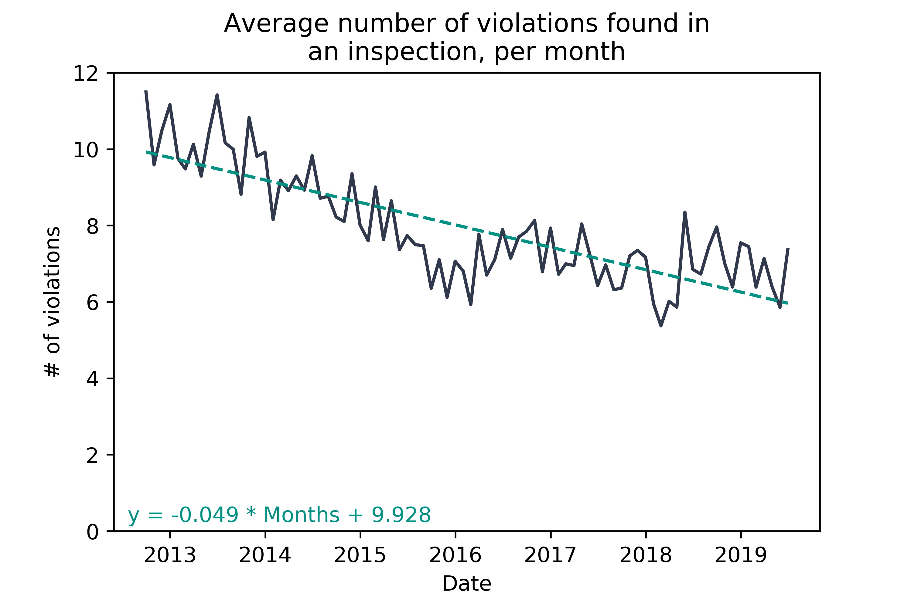There is no trend in average inspection SCORE over time, leading me to think that the change in violations is reporting drift.

Making predictions

Imagine it’s Christmas break, end of 2018, and we’ve scheduled restaurant inspections for the first 6 months of 2019. In hopes of increasing the scores of at-risk restaurants, we’d like to implement a mailing campaign, targeted at restaurants who we expect to receive a low SCORE, giving them information about common violations and advice for proper procedures. Hopefully, this will elicit improvements before our inspector visits, and the restaurant will receive a higher inspection SCORE.

For the purpose of this exercise, we define an “at-risk” restaurant as one we expect to receive a SCORE<93.

Approach

We have data from September 2012 through the end of July 2019. We’re pretending it’s the end of 2019 right now, so January through July 2019 will happen in the “future” and should be ignored during our entire modeling process. They’re the inspections we want to target with the mailing campaign!

The majority of the data before 2019 we’ll use to train our models, leaving a test set of 6 months set aside to see how models would perform out-of-sample. All inspections with an INSPECTDATE prior to 2018-07-01 will be used for training, and the remainder of 2018 will be our test set.

At the very end, we’ll see how our best model would have performed if we actually mailed to the restaurants in the first 6 months of 2019.

Feature engineering

For both the train and test sets, we need inputs from what we know about each restaurant.

Features will include:

• the number of days the restaurant has been open (TIMEOPEN, integer)
• the number of days since the restaurant was last inspected (TIMESINCE, integer)
• the number of other restaurants (unique HSISIDs) with the same name (CHAINCOUNT, integer)
• the number of inspections for the restaurant (INSPCOUNT, integer)
• whether the restaurant has ever needed a re-inspection (WASREINSP, binary)
• the average number of violations per inspection for that restaurant (AVGVIOL, float)

Just for fun and in case of some seasonality to inspections, we’ll throw in cyclical features for month:

• SINMONTH (float)
• COSMONTH (float)

Including preexisting features:

• FACILITYTYPE (categorical and will be converted to dummy variables)
• CITY (categorical and will be converted to dummy variables)
• POSTALCODE (integer, due to the fact that zipcodes that are close in number tend to be geographically similar as well)
• AREACODE (categorical, will be extracted from the existing PHONE NUMBER field

Wrapping in a few details on the restaurant’s most recent inspection, prior to that in question:

• the type of the restaurant’s most recent inspection (TYPE_previous, categorical to dummy)
• the inspector who completed the most recent inspection (INSPECTOR_previous, categorical to dummy)
• the previous inspection score (SCORE_previous, float)

For kicks, we will also use NLP to parse the text in the restaurant’s NAME, in hopes of extracting some insight into the cuisine type or food style (ie. buffet might indicate a higher chance of failing inspection). I’ve arbitrarily decided to choose the top 40 words from restaurant NAME, using most frequent words (most frequent in the training set).

For brevity the entirety of the engineer_features() function has been omitted, but is available in my Example Projects git repository. Here, we’ll simply apply it to the different time windows to create our 3 datasets (X for training, test for testing, and validation to see how our model would’ve done targeting customers in the first half of 2019).

validation_date = '2019-01-01'
test_date = '2018-07-01'

X = engineer_features(insp[insp['INSPECTDATE']<test_date], rest)

validation = engineer_features(insp, rest)
validation = validation[validation['INSPECTDATE']>=validation_date]

test = engineer_features(insp[insp['INSPECTDATE']<validation_date], rest)
test = test[test['INSPECTDATE']>=test_date]

Modeling

We’ll use cross-validation on the X dataset with known scores, to determine optimal model parameters. The reserved test set will be used to choose the best model, hopefully controlling for over-fitting. Finally, we will see how we would perform on the validation set, had we actually implemented the model-building process to identify the 500 most “at-risk” restaurants in the first half of 2019.

Balance classes

The current training set is about 10% “at-risk”, 90% not “at-risk”. To help our models differentiate the two and better identify the most “at-risk”, we’ll adjust the distribution in training by over-sampling our “at-risk” restaurants and mildly under-sampling our not “at-risk”.

oversample = 2 # the number of times to include each positive target row
ratio = .3 # the goal target distribution (% of positive class)

X_neg = X[X['SCORE']<93]
X_pos = X[X['SCORE']>=93]

X = X_pos.sample(int(oversample*len(X_pos)), replace=True).append(
    X_neg.sample(int((1/ratio-1)*oversample*len(X_pos)), replace=True))

Separate input from output

For train, test, and validation we need to separate the target from the input variables.

y = (X['SCORE']<93).astype(int)
X = X.drop(['SCORE', 'INSPECTDATE'], axis=1)

# also separate test, validation into X, and y
y_test = (test['SCORE']<93).astype(int)
X_test = test.drop(['SCORE', 'INSPECTDATE'], axis=1)

y_val = (validation['SCORE']<93).astype(int)
X_val = validation.drop(['SCORE', 'INSPECTDATE'], axis=1)

Make/evaluate a random predictions

We’ll use AUC as our metric of choice for evaluating the model in-sample and out-of-sample. A random prediction should get an AUC of 0.5, and we find that to be true.

from sklearn.metrics import roc_auc_score

print("Train AUC:", roc_auc_score(y, np.random.choice([0,1], size=len(y))))
print("Mailing accuracy:", y_test.loc[np.random.choice(y_test.index, size=500)].mean())

Train AUC: 0.5007870363712852
Mailing accuracy: 0.1

As expected, a random guess produces AUC around 0.5, and only 10% of our mailers, had we randomly chosen 500 inspections in our test set to contact, would have successfully reached an “at-risk” restaurant.

GridSearch for decision tree

Using 3-fold cross validation on the train set, we’ll evaluate a set of parameters to build a decision tree model.

from sklearn.model_selection import GridSearchCV
from sklearn.tree import DecisionTreeClassifier

tree = DecisionTreeClassifier(random_state=1)
tree_grid = GridSearchCV(tree, param_grid={'max_depth':[3,5,7,12],
                                     'max_features':[.5,.8,1.]},
                   scoring='roc_auc', cv=3, n_jobs=-1, 
                         verbose=1, return_train_score=True)
tree_grid.fit(X, y)

tree = tree_grid.best_estimator_

print("Train AUC:", roc_auc_score(y, tree.predict(X)))
print("Test AUC:", roc_auc_score(y_test, tree.predict(X_test)))

tree_mailing_acc = y_test.loc[pd.Series(tree.predict_proba(X_test)[:,1], index=X_test.index).nlargest(500).index].mean()
print("Mailing accuracy:", tree_mailing_acc)
print("Mailing lift:", round(tree_mailing_acc/y_test.mean(), 2))

Train AUC: 0.8119711392149564
Test AUC: 0.7180557838785686
Mailing accuracy: 0.344
Mailing lift: 3.31

We get about a 3x improvement on our mailing performance (over a random guess) by simply using a decision tree - however, the model is over-fit, judging by the drop-off between train and test AUC, and may not generalize well.

GridSearch for bagging

In hopes of combatting overfitting we’ll try bagging, which will allow us to build multiple decision trees on different “views” of the same data. We’ll still use 3-fold cross validation to test different parameters.

from sklearn.ensemble import BaggingClassifier

bags = BaggingClassifier(random_state=1, base_estimator=DecisionTreeClassifier(max_depth=6))
bags_grid = GridSearchCV(bags, param_grid={'n_estimators':[20,120,220],
                                     'max_samples':[.1,.3,.5]},
                   scoring='roc_auc', cv=3, n_jobs=-1, 
                         verbose=1, return_train_score=True)
bags_grid.fit(X, y)

bags = bags_grid.best_estimator_

print("Train AUC:", roc_auc_score(y, bags.predict(X)))
print("Test AUC:", roc_auc_score(y_test, bags.predict(X_test)))

bags_mailing_acc = y_test.loc[pd.Series(bags.predict_proba(X_test)[:,1], index=X_test.index).nlargest(500).index].mean()
print("Mailing accuracy:", bags_mailing_acc)
print("Mailing lift:", round(bags_mailing_acc/y_test.mean(), 2))

Train AUC: 0.76907791565791
Test AUC: 0.7674995890185763
Mailing accuracy: 0.418
Mailing lift: 4.02

This model performs much better overall, with a tiny drop-off between train and test AUC, and superior performance on the mailing compared to the single decision tree.

GridSearch for boosting

For completeness, we’ll try a few more models in hopes of better results - first, boosting, which builds trees on the errors of the previous models, rather than sampling rows like bagging.

from sklearn.ensemble import GradientBoostingClassifier

boost = GradientBoostingClassifier(random_state=1, init=DecisionTreeClassifier(max_depth=6))
boost_grid = GridSearchCV(bags, param_grid={'n_estimators':[20,120,220],
                                            'max_features':[.3,.5,.8]},
                   scoring='roc_auc', cv=3, n_jobs=-1, 
                         verbose=1, return_train_score=True)
boost_grid.fit(X, y)

boost = boost_grid.best_estimator_

print("Train AUC:", roc_auc_score(y, boost.predict(X)))
print("Test AUC:", roc_auc_score(y_test, boost.predict(X_test)))

boost_mailing_acc = y_test.loc[pd.Series(boost.predict_proba(X_test)[:,1], index=X_test.index).nlargest(500).index].mean()
print("Mailing accuracy:", boost_mailing_acc)
print("Mailing lift:", round(boost_mailing_acc/y_test.mean(), 2))

Train AUC: 0.6919756499060097
Test AUC: 0.6839333662118472
Mailing accuracy: 0.42
Mailing lift: 4.04

A solid model, but much lower AUC, both in-sample and out-of-sample.

GridSearch for random forest

Lastly, we’ll try a random forest, which samples both features (like boosting) and rows (like bagging).

from sklearn.ensemble import RandomForestClassifier

rf = RandomForestClassifier(random_state=1, max_depth=6)
rf_grid = GridSearchCV(bags, param_grid={'n_estimators':[20,120],
                                     'max_samples':[.3,.5,.7],
                                     'max_features':[.3,.4,.5]},
                   scoring='roc_auc', cv=3, n_jobs=-1, 
                         verbose=1, return_train_score=True)
rf_grid.fit(X, y)

rf = rf_grid.best_estimator_

print("Train AUC:", roc_auc_score(y, rf.predict(X)))
print("Test AUC:", roc_auc_score(y_test, rf.predict(X_test)))

rf_mailing_acc = y_test.loc[pd.Series(rf.predict_proba(X_test)[:,1], index=X_test.index).nlargest(500).index].mean()
print("Mailing accuracy:", rf_mailing_acc)
print("Mailing lift:", round(rf_mailing_acc/y_test.mean(), 2))

Train AUC: 0.6950166305726755
Test AUC: 0.6854402980985259
Mailing accuracy: 0.426
Mailing lift: 4.1

Comparable to boosting alone, and still not as good as bagging.

Simulating the mailer

We selected our bagging model as the winner during the modeling process. Now, let’s use it to predict the inspections in the first half of 2019, and “see the future” to see how we would’ve done.

y_val.mean()

0.0989065606361829

Remember, if we randomly mailed to restaurants about to be inspected we could expect only 9% of the recipients to be designated “at-risk”.

y_val.loc[pd.Series(bags.predict_proba(X_val)[:,1], index=X_val.index).nlargest(500).index].mean()

0.412

However, if we used the bagging model that won during modeling, we would’ve successfully contacted 41% “at-risk” restaurants!

Code

Complete code can be found in my Example Projects git repository.

Project primarily relied on pandas, sklearn, with some matplotlib, numpy, and re.

Please note that part of this work was submitted as part of a technical interview for NetApp, but the method, code, and commentary contained/described herein is my own independent work and has been adapted/published with permission.