Playing 2048 with AI - pt. 2
Series recap
2048 is a game where the player chooses one of 4 actions to move the tiles in (up, left, down, and right), when presented with a board layout, to combine tiles until they reach a value of 2048 (or larger). Part of a game would look like:
Our desired end result in this series is a neural network which can consistently achieve the 2048 tile, when given a new game. To achieve this, we will allow the network to repeatedly attempt different strategies, “learning” from each game’s results until its performance improves.
My implementation of the game logic, using only numpy, is described in the previous post in this series.
Formulation
Let’s take a moment to remember our goal - we want a neural network that will accept a mathematical representation of a board layout, and will produce a probability distribution, representing what the best move(s) are.
Let’s generally represent a board layout mathematically as a vector, \(L\). This layout should be passed into a model, which outputs a probability distribution (let’s call it \(\hat{Y}\)) for the 4 moves (up, left, down, and right, respectively). Ignoring the linear algebra that happens inside the model, generally \(model(L)=\hat{Y}\).
To illustrate, here’s an example board layout:
[ 0,16, 8, 0,
  2,32, 4, 0,
  0, 0, 8, 0,
  0, 0, 0, 0]
For this toy layout, maybe it would be \(model(L)=\hat{Y}=[.1,.2,.6,.1]\), indicating the model thinks the best course of action is to swipe down (with 60% confidence), followed by left (20% confidence) and either up or right (both with 10% confidence).
Choosing moves
We could simply choose the move with highest probability (for our toy layout, we’d swipe down). However, if we introduce more randomness at this stage, the network will attempt a wider variety of moves given the same layout, hopefully discovering better strategies. To accomplish this, we’ll draw a random sample of size 1 from this probability distribution. Let’s call this \(X : \hat{Y} \rightarrow M\), where \(M\) is a vector indicating the move selected.
Continuing our toy example, say \(X([.1,.2,.6,.1])\) outputs [0,1,0,0], indicating that the computer chose the second highest probability option (chose to swipe left).
So now we know the layout (\(L\)), what distribution the computer recommended (\(\hat{Y}\)), what action was taken (\(M\)), and eventually (given several more moves/decisions) we’ll know the result of the game.
Finding \(Y\)
Typically, when training any machine learning model, you have a set of known, correct labels, commonly referred to as \(Y\), and you repeatedly train the model until \(\hat{Y}\) (the recommendation produced by the model) gets sufficiently close to \(Y\), using whatever loss function you’ve selected. In more simple terms, we know what labels we want the model to produce, and train it until it consistently produces them. In reinforcement learning, there are no correct labels. We don’t know, given our toy layout, what the best move is, we only know the results of the entire game. How do we train?
Moving away from math for a moment, we want our neural network to perform more moves like those that resulted in “good” games, and fewer moves like those that resulted in “bad” games.
I’ll now define \(Y=f(M, game)\), where \(f\) maps the move that was chosen and the overall game performance to a probability distribution for the 4 different move options (up, left, down, right) that, during training, should encourage \(\hat{Y}\) to approach \(M\) if the game was “good”, and diverge from \(M\) if the game was “bad”.
I’ve chosen to define \(f(M, game)\) as follows: \[Y = f(M, game) = \begin{cases} M &\text{if } \text{\textquotedblleft}good\text{\textquotedblright} game \\ (1-M)/3 &\text{if } \text{\textquotedblleft}bad\text{\textquotedblright} game \end{cases}\]
Let’s illustrate this by looking at our toy example again.
Given our layout \(L\), we had \(model(L)=\hat{Y}=[.1,.2,.6,.1]\). We also already randomly selected from this distribution, choosing to swipe left, using \(M=X(\hat{Y})=X([.1,.2,.6,.1])=[0,1,0,0]\).
If this was a “good” game, we want to perform more moves like \(M\), so \(Y=M=[0,1,0,0]\). In English, this is the same as telling the model “yes, always swipe left in this situation!”
If this was a “bad” game, we don’t want to make a move like \(M\), but we don’t know what move would be better, because we never played out that scenario. So \(Y=(1-M)/3 \approx [.33,0,.33,.33]\). In English, this is the same as telling the model “Not left, but I don’t know which direction to swipe instead…”
I’ll discuss how I separated “good” and “bad” games later in this post.
Loss
Now we have \(Y\), we need to tell the network how to adjust its weights with some objective function in mind, so that \(\hat{Y}\) slowly approaches \(Y\). I’ve decided to train to minimize Mean Absolute Error (L1 loss), which calculates the average distance between \(\hat{Y}\) and \(Y\) for a single move: \[Loss(Y, \hat{Y})=\sum_{i=0}^4 |\hat{Y_i}-Y_i|/4\]
For this toy example \(\hat{Y}=[.1,.2,.6,.1]\), if the game was “good” and \(Y=M=[0,1,0,0]\), the network would calculate loss as: \(\frac{|.1-0|+|.2-1|+|.6-0|+|.1-0|}{4} = 0.4\). To decrease this, the network should adjust model weights to increase the probability of swiping left, and decrease the probability of swiping in any other direction, given our layout \(L\).
If the game was “bad” and \(Y=(1-M)/3=[.33,0,.33,.33]\), our loss would be: \(\frac{|.1-.33|+|.2-0|+|.6-.33|+|.1-.33|}{4} = 0.2325\). To decrease this, the network should adjust model weights to decrease the second term (probability of swiping left), while equalizing the others.
Weighting loss
Currently, we evaluate each move individually, and each move contributes equally to the overall loss (and, therefore, the direction to update the model weights). This is probably not ideal, and I decided to manually weight my loss function in hopes of helping the network learn by (hopefully) reducing some of the random noise from less-important phases of games.
Problem #1 - good and bad games
Currently, we have a binary divide between arbitrarily-defined (later in this post) “good” and “bad” games, but I want be able to differentiate how good or bad a game was. I would prefer for moves associated with “very good” games contribute more to how the network adjusts than “mediocre” games. Similarly, “very bad” games should contribute more than “sub-par” games.
For example, a game that achieves the same goal (perhaps a tile of value 2048) in fewer moves should be “better” than one that achieves that goal in more moves, though both are “good” and would use \(Y=M\). Alternatively, maybe a game that achieves 2048 with a higher score is better than another “good” game which also achieved 2048, but with a lower score.
In order to control this first issue, I’ll sometimes be adding a weighting at the game level. Going forward I’ll refer to this as game-level weight \(j\), and it should range [0,1]. I’ll use different methods to calculate \(j\), but it will always be designed to capture shades of how “good” the game was. Every move in a single game will have the same \(j\), but \(j\) varies between games.
I’ll discuss the different game-level weighting techniques later in this post.
Problem #2 - importance of moves
We currently treat each move within a game as equally important, but it may be that some moves contribute more to the overall game’s performance than others. For example, moves towards the end of the game are probably more important than moves at the start (does which direction you initially swipe really have an impact on the full game?). Alternatively, moves when the board is crowded (has many non-zero tiles) probably matter more than when the board is relatively clear, as the risk of getting “stuck” and the game ending is higher.
In order to control this second issue I’ll also sometimes add a move-level weight, \(k\). It will be designed to differentiate moves in the same game, ranging from [0,1] to designate how “important” that individual move is to the overall game performance. Note that moves in a single game will have different \(k\) values.
I’ll discuss the different move-level weighting techniques later in this post.
So my final weighted L1 loss is actually \[Loss(Y, \hat{Y})=\sum_{i=0}^4 j*k*|\hat{Y_i}-Y_i|/4\]
Everything’s relative
Before moving forward, I’d like to take a moment to discuss the batch process I decided to use during training. Each game that the network plays could change when the model parameters change, or just due to the random nature of the game, so I decided to constantly update my dataset. Every “epoch”, the network was trained on a slightly different set of games.
Fundamentally the process looked like: use the model to run some number (batch_size) of games, use games to change model, run another batch of games, train with both batches, etc. until hitting the forget_interval, which is the number of epochs each batch of games will be used in. From that point onward, we have a rolling window where each epoch considers forget_interval number of games, which would look like:
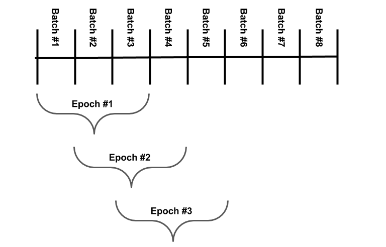
Also worth noting, is that since my games are different each epoch, I felt it unwise to set an absolute metric for measuring both \(j\) and \(k\), and instead chose to measure each game/move relative to the others in its epoch. My logic here was a “good” game early during training (perhaps reaching the 128 tile) would actually be quite a poor game later in training (perhaps when most games are reaching the 1024 tile).
Weighting
I previously mentioned that I would include a \(j\) and \(k\) term in my loss function, to capture the strength of “good”/”bad”-ness in a game, and importance of individual moves within a game, respectively. Here, I will expand on the options I decided to code for each.
Defining “good” and “bad”
As discussed in the previous section I used relative metrics for classifying games as “good” or “bad” - generally, each is defined as “good” if it performed better than the epoch’s median performance, and “bad” if it performed equal to or below the epoch’s median. This performance is measured using the same metrics that I use to calculate \(j\), and by default uses scores. Let’s discuss these metrics now.
Defining \(j\)
This term defines the strength of how “good” or “bad” an overall game is, relative to its batch, and ranges [0,1].
I rank with a few different metrics as options:
scores- the final score accumulated during the gamemax- the maximum tile achieved at the end of the gamelog2_max- the base 2 log ofmaxThis approach equalizes the distance between each new tile value, while
maxwould over-weight later tile upgrades and under-weight earlier (for example, making it from 1024 to 2048 would matter a lot more than making it from 124 to 248), and this may not always be desirable.tile_sums- the sum of all tiles remaining on the board at the end of the game/
By default, I used scores.
“Good” and “bad” games are transformed separately, using these metrics and the median to find how close each “bad” game is to the “worst” in its epoch, and each “good” game is to the “best”. Closer to the median means closer to \(j=0\), while closer to the outlier means closer to \(j=1\).
This is all defined in compute_game_penalties(...), for those looking at code.
Defining \(k\)
This term defines how important a single move is to the overall game that contains it.
By default, I again used uniform weighting, with all moves equally important at \(k=1\).
For more granularity, I again rank using different metrics:
nonzero- the fraction of tiles that are nonzero when that move is made (out of 16)linear_move_num- how close the move is to the end of the game, calculated by move # divided by the total number of moves in that gameexponential_move_num- also how close the move is to the end of the game, but increases exponentially following \(1-e^{-3x}\) where x islinear_move_num
This is all defined in compute_move_penalties(...), for those looking at code.
Controlling randomness
We already have randomness in the training process, as \(X\) performs a random sample using probabilities defined by \(\hat{Y}\) to select the computer’s move each turn. However, I wanted the option to inject more randomness into the process, and so included two other parameters to my train(...) function.
random_games is simply a boolean, that runs the same batch_size number of entire games with a completely even probability distribution, allowing the computer to see what pure random chance would produce in the same scenario.
random_frac instead is a float ranging [0,1], that indicates what fraction of each game’s moves should be completel random. For example, with random_frac=.1, the network itself would perform 9/10 moves on average, and the other move would be randomly generated, interjecting more noise in the training process.
Theoretically this additional randomness would be more useful at the start of training, and less useful towards the end, as the random games do not improve over training as the network should. Eventually (assuming the network is able to learn successfully), the network-run games would all outperform the completely random games, and it may slow training at the end as the network continues to penalize the “bad” games that it did not produce. However, I felt it interesting to include, thinking the network performance might get “stuck” performing similar strategies over and over, and providing the network a look at more random strategies could help un-stick it.
More advanced training would allow for toggling both of these during later epochs, as the model performs better, but I have prioritized getting results rather than adding yet more parameters to tune.
Actually training
Now all the heavy lifting has been done, I’ll take a moment to describe some code, though all of it is available in my repository for this project.
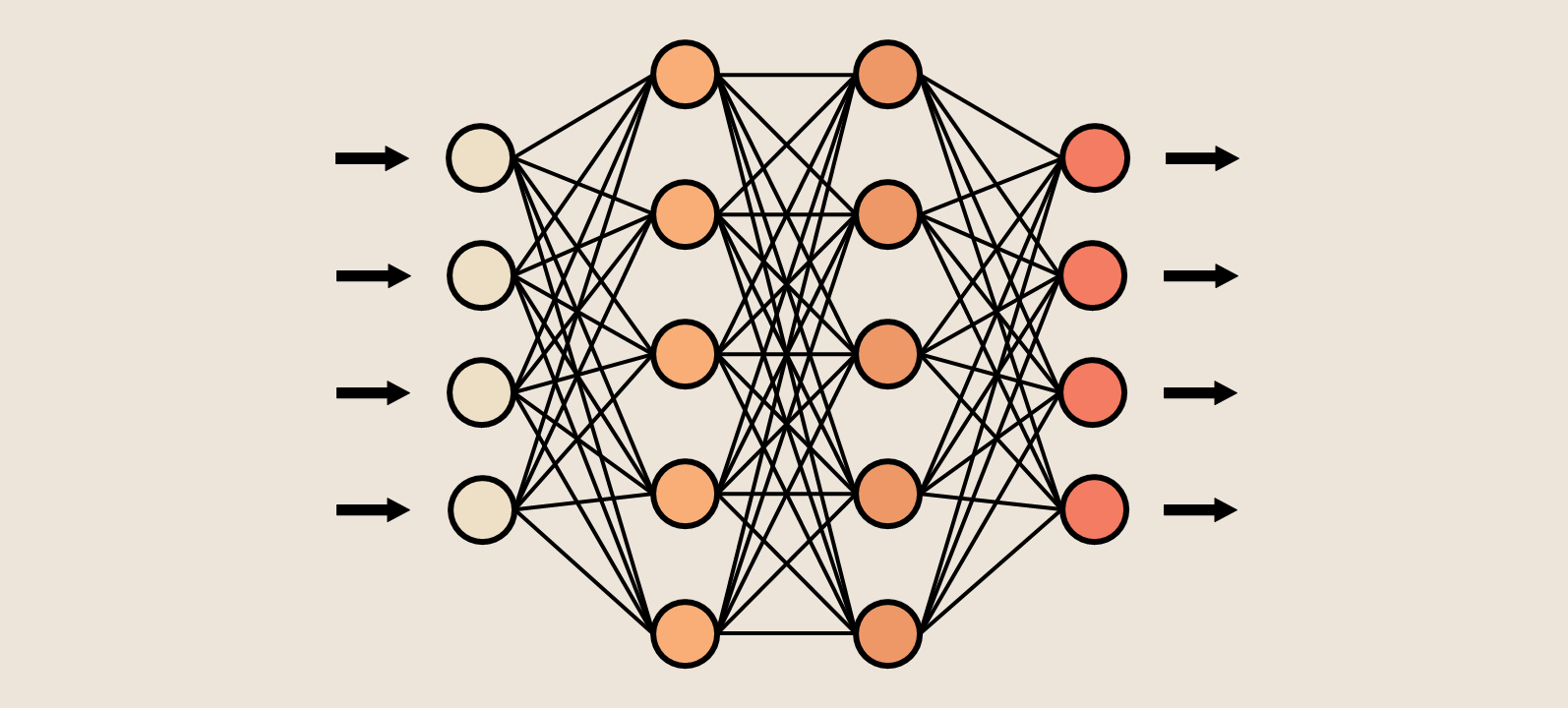
The network itself is built using pytorch, and I leveraged their implementations of the Adam optimizer and L1Loss, as follows:
class NeuralNetwork():
    def __init__(self, inputSize=16, outputSize=4, neuronCountJ=200, neuronCountK=100):
        # initialize network
        self.model = torch.nn.Sequential(nn.Linear(inputSize, neuronCountJ),
                       torch.nn.ReLU(),
                       torch.nn.Linear(neuronCountJ, neuronCountK),
                       torch.nn.ReLU(),
                       torch.nn.Linear(neuronCountK, outputSize),
                       torch.nn.Softmax(dim=1),
                     )

		self.opt = torch.optim.Adam(model.parameters(), lr=1e-3)
		self.loss = torch.nn.L1Loss()
All the logic previously described is triggered by calling the NeuralNetwork.train(...) function. All the other functions support this main functionality, of running a large number of games/mini-games and training a single network.
Final parameter list
random_games: either True or False, described earlier hererandom_frac: either None or a float ranging[0,1], described earlier herebatch_size: any integer greater than zero, described earlier hereforget_interval: any integer greater than zero, described earlier herelr: the learning rate for the network, defaults to 0.001move_penalty_type: choose from[None,'nonzero','linear_move_num','exponential_move_num'], described earlier heregame_penalty_type: choose from['scores','max','log2_max','tile_sums'], described earlier here
Results
After (more than a few) days of attempting to parameter tune without seeing much in the way of performance improvement, I finally realized what, perhaps, I should’ve realized before putting so much work into this project - the level of complexity in this game will make it infeasible for me to test my implementation.
On average, a completely randomized game of 2048 will require over 100 moves to complete and get any measure of performance. As games improve, the number of moves required will only increase, making it more and more difficult to attribute overall performance to individual moves. I can only imagine the error surface that my poor network would be traversing.
Proof of concept
However, I set myself the small goal of training a network to perform the first 20 moves of a game, hoping to see the network become more efficient at scoring points, with a tightly limited scope.
Plotted below, you can see each batch’s average score after 20 moves, by training epoch. You can see the initial, random games start with about a final score of 85.4 after 20 moves. I set the program to cut off after a batch reached an average final score of 87 or training duration hit 3 hours, whichever came first.
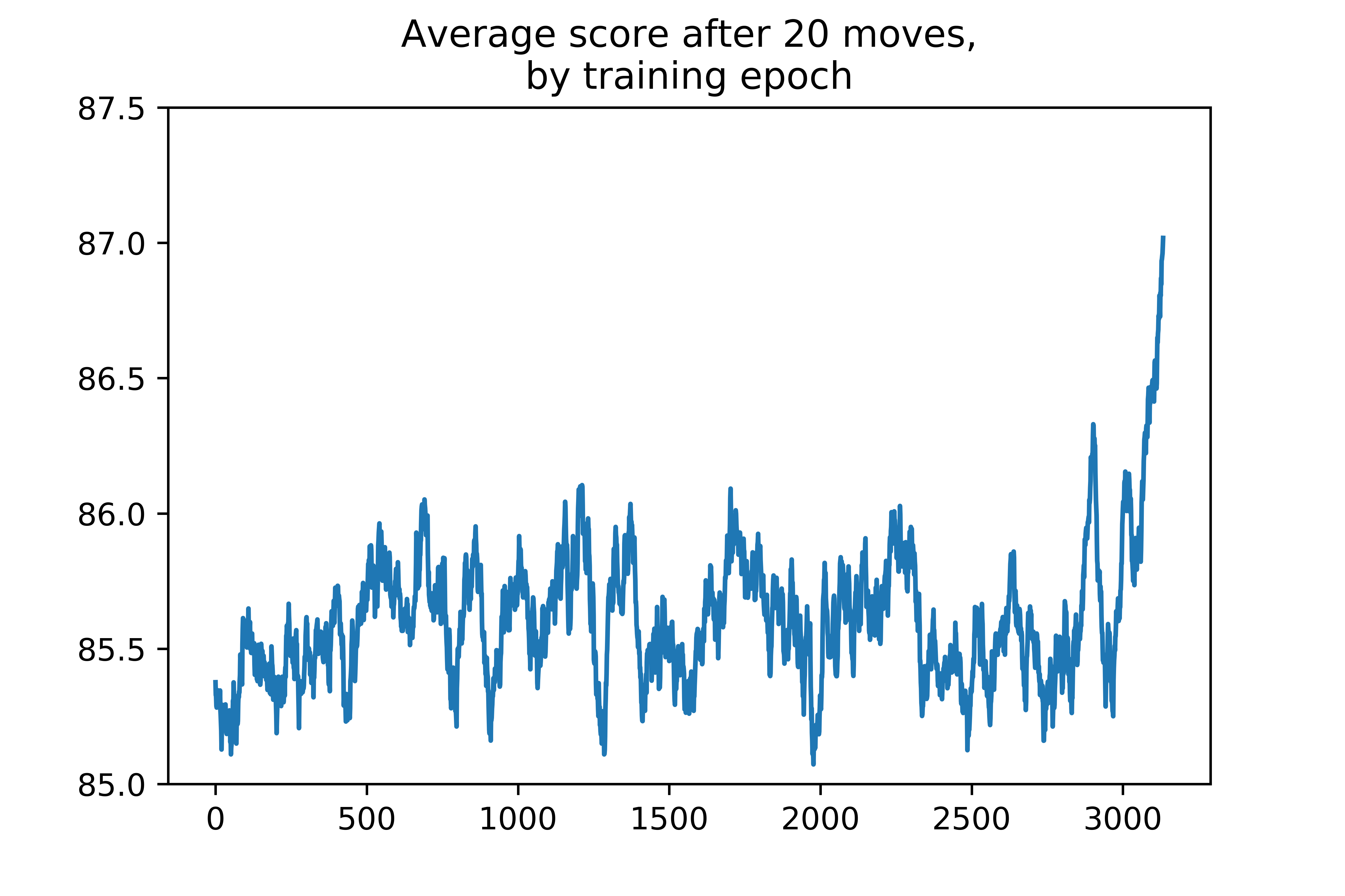
This is a promising result, but I have little enthusiasm for it. It took about 2.5 hours for the network to achieve an average score of 87, completing a <2% performance improvement over only the first 20 moves of the game. I can only guess how much training time would be required to see comparable improvement for entire games.
Final thoughts

I wish I had the resources to pursue this project further, but I post this work proudly.
When I set out to do this project, I wanted to study reinforcement learning. I also wanted to use Pytorch for the first time, practice object-oriented programming, and try binder.
As ever, the goal of this blog is to increase my own knowledge base, which I can confidently say this project has.
Code
Complete code can be found in my 2048 git repository.
This section of the project relies on numpy and pytorch 1.1.0. Additional packages (such as widgets and matplotlib) may be required to run any notebooks in the repository.