Recommending TV Shows via Collaborative Filtering

Challenge
Imagine you are Netflix, Hulu, or any other streaming site that has to recommend new shows. Your goal is to recommend a new show only to those users who will enjoy it, so a big part of your product is the ability to measure a user’s tastes, and predict how much they will like new things.
In this post, I’ll demonstrate a common technique used in recommendation engines: collaborative filtering.
Algorithm overview
So what is collaborative filtering? Simply put, it is a technique to predict a person’s interest in a product, based on similar users’ preferences.
Typically, the most basic way to predict a new user’s affinity for a product is to look at how everyone else likes it. The base assumption in collaborative filtering is if two users have the same opinions on some known products, then the users are likely to share opinions on other things, like new products.
The technique isn’t limited to a single algorithm, but rather is made of a whole family of similar approaches, that generally consist of:
- A method to decide how “similar” different users are, based on their preferences
- A method to combine “similar” users’ preferences to create the prediction
The technique is simple, and can be applied to a broad range of problems. Some potential use-cases are:
- Whether a person will buy a new brand of cereal
- Which of political candidate the person more likely to vote for
- How a person would rate a new TV show
In this post, I’ll demonstrate one approach to the third use-case. My goal will be to, as accurately as possible, predict a user’s interest level in a new show.
Dataset
In this exercise I’ll use a set of 0-10 ratings users have given shows on the website MyAnimeList. The dataset is available on Kaggle.
I’ll be focusing on the “filtered” dataset available on Kaggle, simply to reduce the volume of data.
Initializing the data
It’s important to note here that, traditionally, collaborative filtering only considers a user’s behavior, rather than “who” they are. This would mean that the dataset could consist of how the user rated certain shows, whether they clicked certain links, whether they bought certain items, or how much time they spent on certain pages. The dataset would not include information like the user’s age, gender, ethnicity, or the country they reside in.
In our dataset, we will only look at the users and the ratings they gave to shows, which are contained in animelists_filtered.csv. As I’m doing this analysis on a laptop, I’ll also be limiting the number of shows.
import pandas as pd

reviews = pd.read_csv('animelists_filtered.csv', nrows=200000,
			usecols=['username', 'anime_id', 'my_score'])

# downsample to a complete set of reviews for a subset of shows
reviews = reviews[reviews['anime_id'].isin(reviews['anime_id'].unique()[:-1])]

# pivot for one row per user, and column per anime
reviews = pd.pivot_table(reviews, index='username',
			columns='anime_id', values='my_score', aggfunc=max)
Looking at our dataset, we have the “classic” collaborative filtering layout: one row per user, with their preferences (in this case, a rating 0-10) for each show in each column.
| username | 21 | 59 | 74 | 120 | 178 | 210 | 232 | 233 |
|---|---|---|---|---|---|---|---|---|
| cornivious | 0.0 | 0.0 | ||||||
| Acid | 10.0 | 7.0 | 8.0 | 8.0 | ||||
| xDivinityXD | 10.0 | 9.0 | 10.0 | 10.0 | 10.0 | 10.0 | ||
| Seismic | 8.0 | 8.0 | ||||||
| AkatsukiUlquiora | 0.0 | 9.0 | 0.0 | 0.0 | 10.0 | 9.0 | 10.0 | 0.0 |
Defining the targets
One of the best parts of collaborative filtering is that the technique is target-agnostic - once you determine who similar users are, you can map any one of their preferences onto the others.
In the spirit of this, I will demonstrate using the same filtering algorithm to predict three different shows: by index they are [210, 232, 233], but by name they are Ranma ½, Cardcaptor Sakura, and Daa! Daa! Daa!.
Looking at how users have rated the shows:
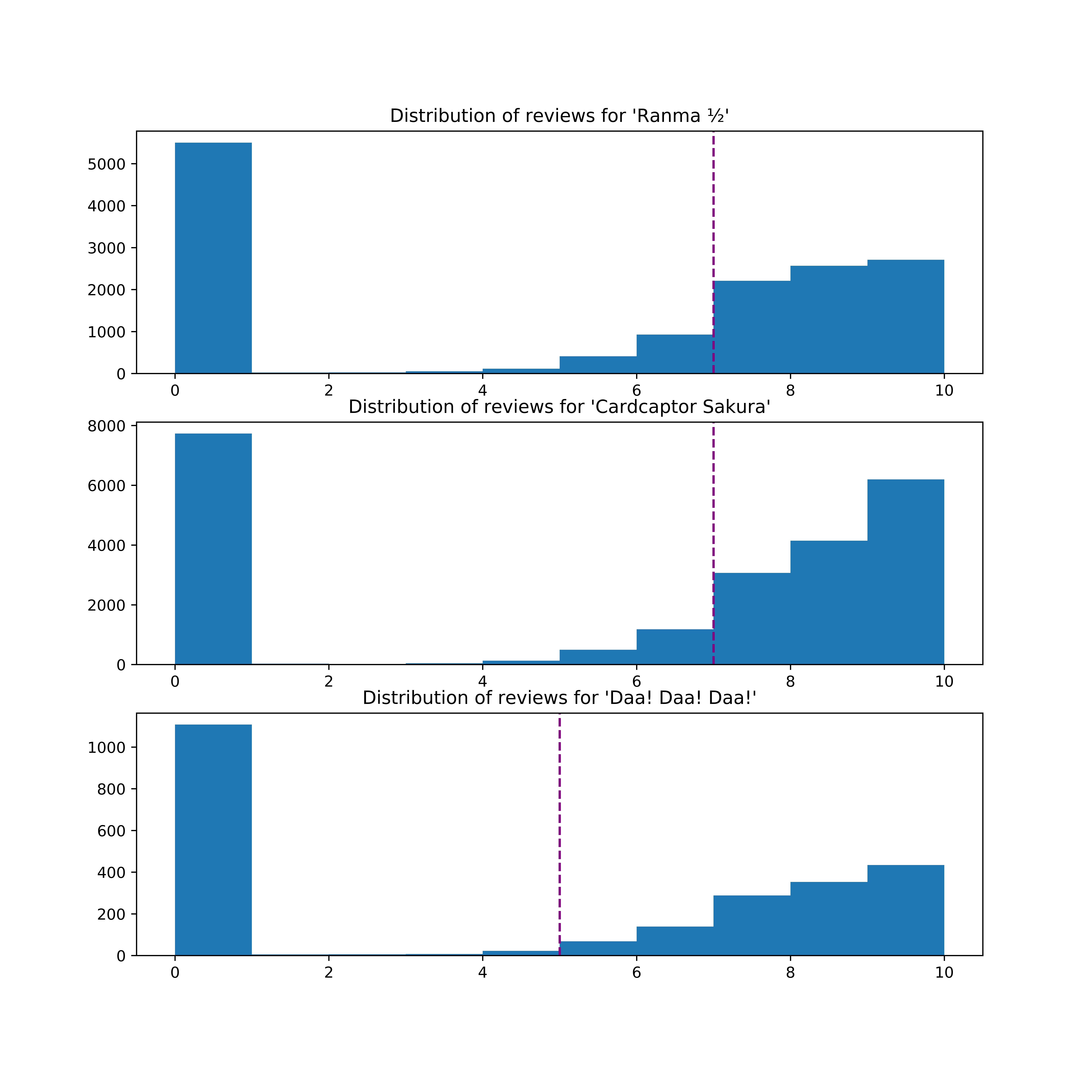
We can see an interesting pattern across all three shows, where the majority of people who bother to rate a show do so to assert their dislike of it (hense the spikes at zero). Everybody else offered a little more granularity, with most people really liking it and a long tail towards 0.
I’ve also marked the median rating for each show, in purple.
Also of note are the different y axes, as the scales differ. A lot more people have watched Cardcaptor Sakura than have watched Daa! Daa! Daa!.
Splitting the data
I’m going to randomly assign 30% of the users to the test set, or the “unknown” users - those whose ratings of our target shows we will attempt to predict, and to gauge the algorithm’s accuracy.
from sklearn.model_selection import train_test_split

train, test = train_test_split(reviews, test_size=.3, random_state=1)
Defining success
As my metric I’ll use mean absolute error, which can be interpreted as how many points (out of 10) the average prediction differed from that user’s true rating of the target show. I selected this metric over the more common root-mean-square error, as RMSE tends to over-weight outliers and, due to the spike at zero, I prefer to avoid averages.
Accuracy baseline
Our goal is to predict the test users’ ratings of our target shows, using only information we can gather from the train users’ behavior. What would be the most basic method we could do?
Usually, an average or median approach are a data scientist’s first stop, so we’ll attempt a median. Again due to the spike at zero for each show, the average will be pulled down, and it’s a better idea to use a method that doesn’t over-weight the edges of the distribution where users didn’t bother to rate the show beyond a binary “I didn’t like it”.
Since we’re ignoring the test set, we can find the median of the training set for each show:
| Median rating | |
|---|---|
| Ranma ½ | 7.0 |
| Cardcaptor Sakura | 7.0 |
| Daa! Daa! Daa! | 5.0 |
Implementing it, we simply want to know the mean absolute error between these medians and every test user’s rating of the show (if they rated it).
from sklearn.metrics import mean_absolute_error

for target_col in target_cols:
    score = mean_absolute_error(test[target_col].dropna(),
                    np.repeat(train[target_col].median(), test[target_col].notna().sum()))
| Test error (median approach) | |
|---|---|
| Ranma ½ | 3.47 |
| Cardcaptor Sakura | 3.37 |
| Daa! Daa! Daa! | 3.82 |
We have our baselines! Hopefully, any collaborative filtering approach we take from here will reduce these errors.
Collaborative filtering
Given our baseline approach is the median, we now want to use the baseline as a starting point, and update the prediction for each user, based on how users who are similar to them liked the target show.
Finding similar users
Our first priority is to identify users who respond to shows in a similar way. Any number of similarity/distance metrics could be used here, but I’ll be using a centered cosine similarity (also known as the Pearson correlation coefficient).
Let’s look at a quick example to see how this works.
Demo
| Show A | Show B | |
|---|---|---|
| User A | 6 | 7 |
| User B | 6 | 3 |
| User C | 1 | 1 |
| User D | 4 | 8 |
| User E | 8 | 3 |
| User F | 2 | 4 |
Plotting the users’ two-dimensional preferences, we can see a wide spread.
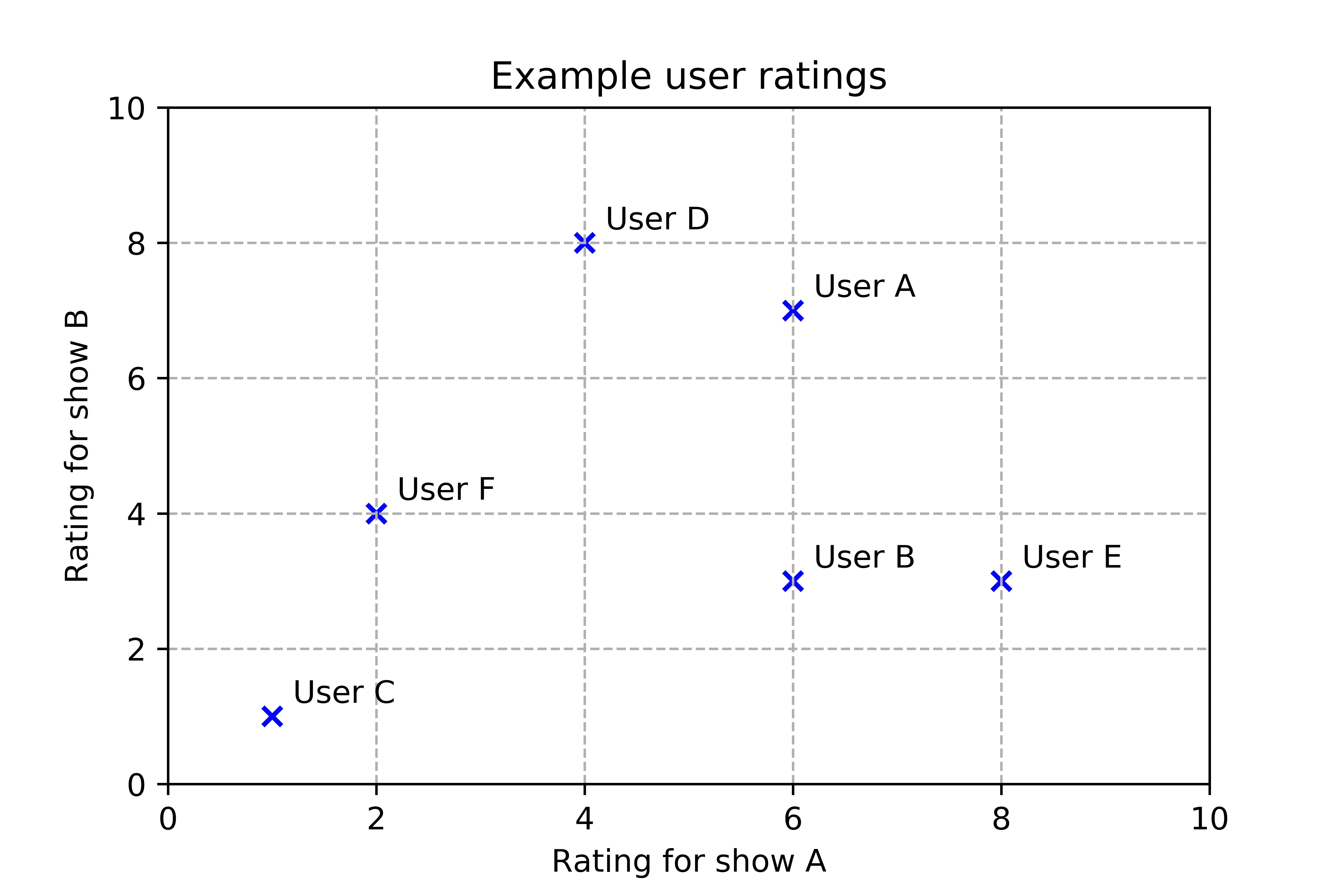
Euclidean distances or any other similarity metric could work here, but what I am interested in doing is determining directionality, or rather finding users whose preferences vary in similar ways, so as to update the unknown users’ preferences based on how the known users’ varied on that show. Stay with me.
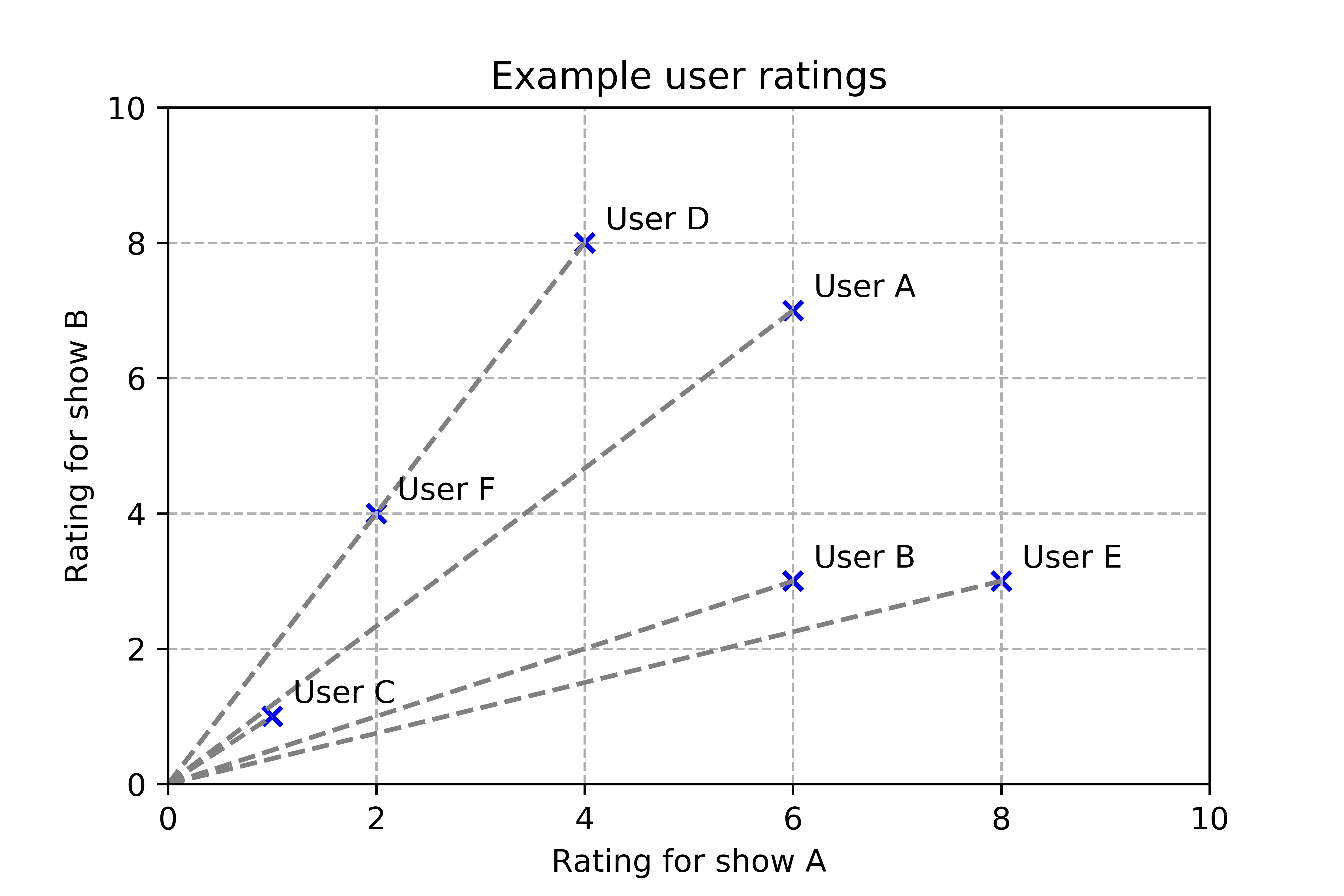
If I was using euclidean distance, User D would be most similar to User A. Instead, using cosine similarity, I can say that User D likes Show B twice as much as they like Show A, and so does User F. They are perfectly similar, using directionality!
Now, how about the “centered” part of the metric? All that means is, insead of comparing a user’s base preferences, we compare the change between their average preference and their show-specific preference.
Let’s include an extra
| Show A | Show B | Average | Prediction show | |
|---|---|---|---|---|
| User D | 4 | 8 | 6 | 5 |
| User F | 2 | 4 | 3 | ? |
We’ve already said that User D is perfectly similar to User F, while User D has rated the prediction show, and User F hasn’t. We can now predict that User F will give the prediction show a rating of 2.
Why? Because the two users are similar, and User D liked the prediction show 2 rating points less than they like shows on average. Following our initial assumption that similar users have similar tastes, we can logically conclude that User F will like the prediction show 2 rating points less than they like shows on average (4 points).
Implementation
Let’s see it in action!
Our first step is to separate the target columns from the others. We will completely ignore them for now, while we calculate similar users with the ratings for other shows.
train_targets = train[target_cols]
test_targets = test[target_cols]

train = train.drop(target_cols, axis=1)
test = test.drop(target_cols, axis=1)
Now, we want to zero-center our datasets (saving the means for later adjustments).
train_mean = train.mean(axis=1)
test_mean = test.mean(axis=1)

train = train.apply(lambda col:col-train_mean)
test = test.apply(lambda col:col-test_mean)

train_targets = train_targets.apply(lambda col:col-train_mean)
test_targets = test_targets.apply(lambda col:col-test_mean)
Finally, we’ll fill nulls with zero (to ignore directionality from shows without ratings), and actually find similar users, using scikit-learn’s cosine_similarity class.
from sklearn.metrics.pairwise import cosine_similarity

sim = pd.DataFrame(cosine_similarity(train.fillna(0), test.fillna(0)),
                   index=train.index, columns=test.index)
So what does sim look like? It has one row per known user, and one column per unknown user. Each value is the similarity between the two on a [-1,1] scale, where 1 indicates highly similar, and -1 indicates not similar at all.
| anthony6467 | mateuszek | Lawlieth | ChronoKid | Laurentius | |
|---|---|---|---|---|---|
| sakurabana | 0.0 | 0.0 | 0.0 | 0.0 | 0.0 |
| WireRabbit | 0.0 | 0.0 | 0.0 | 0.0 | 0.0 |
| ayami123 | 0.0 | 0.645497 | 0.866025 | -0.327327 | 0.0 |
| kawaiiteen | 0.0 | -0.223607 | 0.0 | -0.755929 | 0.0 |
| shimo0712 | 0.0 | 0.0 | 0.0 | 0.0 | 0.0 |
In this excerpt of the data, we can see that our unknown user Lawlieth is highly similar to known user ayami123, so we could use the taste profile from ayami123 to determine how Lawlieth will respond to the target shows!
Combining similar users’ preferences
The most basic example, which we went through in the demo, involves finding the most similar known user according to directionality, how the most similar user’s rating on the target show differed from their average rating, and then using that difference to find how the unknown user’s rating on the target show would differ from their average rating.
Let’s do that now.
def find_adjustment(target_col, sim, unknown_user, train_targets):
    most_similar_known_user = sim[unknown_user].idxmax()
    known_user_adjustment = train_targets.loc[most_similar_known_user, target_col]

    return known_user_adjustment

prediction = test_mean.loc[unknown_user]+find_adjustment(target_col, sim,
							unknown_user, train_targets)
Another alternative is to combine multiple adjustments, perhaps a set number of them and finding the average adjustment:
def find_adjustment_n_users(target_col, sim, unknown_user, train_targets, n):
    most_similar_n_users = sim[unknown_user].nlargest(n).index
    known_users_adjustment = train_targets.loc[most_similar_n_users, target_col].mean()

    return known_users_adjustment

prediction = test_mean.loc[unknown_user]+find_adjustment_n_users(target_col, sim,
							unknown_user, train_targets, n)
Ultimately, the calculated adjustment is still used to adjust the unknown user’s average rating.
Evaluation
| Median approach (baseline) | Single user CF | 25 users CF | Baseline improvement | |
|---|---|---|---|---|
| Ranma ½ | 3.47 | 3.36 | 2.95 | 14.9% |
| Cardcaptor Sakura | 3.37 | 3.13 | 2.82 | 16.2% |
| Daa! Daa! Daa! | 3.82 | 2.83 | 2.58 | 32.5% |
It’s beautiful! Using just 25 similar users, we can noticeably improve our predictions.

Conclusion
You might be thinking that collaborative filtering isn’t that accurate, and you might be right. However, it is computationally efficient (as we only needed to calculate similarities once), and can be applied to a wide variety of problems. It is a great basis for any recommendation engine, especially if you’re dealing with a large volume of sparse data.
Bonus: dataset reduction
One of the best parts of collaborative filtering is you don’t have to remember every data point, but can instead combine, simply remembering how many users shared that set of preferences.
Remember, our original dataset of reviews looked like this:
| username | 21 | 59 | 74 | 120 | 178 | 210 | 232 | 233 |
|---|---|---|---|---|---|---|---|---|
| cornivious | 0.0 | 0.0 | ||||||
| Acid | 10.0 | 7.0 | 8.0 | 8.0 | ||||
| xDivinityXD | 10.0 | 9.0 | 10.0 | 10.0 | 10.0 | 10.0 | ||
| Seismic | 8.0 | 8.0 | ||||||
| AkatsukiUlquiora | 0.0 | 9.0 | 0.0 | 0.0 | 10.0 | 9.0 | 10.0 | 0.0 |
On my system, I was storing 29,782 rows, worth 2.14 MB of data. Not huge, but I’m working on a laptop and this is just a demonstration. In true production, data sizes would explode.
If instead we group by the values (known and unknown), store the number of users who had that combination for the in-sample shows, and stored the average for the target shows, we don’t need anything else!
reviews.loc[:,non_targets] = reviews.loc[:,non_targets].fillna(-1)

reviews = pd.concat([reviews.groupby(non_targets)[target_cols].mean(), reviews.groupby(non_targets).size().rename('weight')],
          axis=1).reset_index().replace(-1, np.nan)
Now, the dataset looks like:
| 21 | 59 | 74 | 120 | 178 | 210 | 232 | 233 | weight |
|---|---|---|---|---|---|---|---|---|
| 0.0 | 3.777778 | 5.542857 | 4.333333 | 43 | ||||
| 2.0 | 4.500000 | 2 | ||||||
| 4.0 | 8.000000 | 6.000000 | 2 | |||||
| 5.0 | 5.600000 | 3.500000 | 5 | |||||
| 6.0 | 8.000000 | 7.666667 | 3 |
Admittedly, we have forgotten who is who, but if we just want to know who a new user is most similar to using collaborative filtering, we need the preferences, not the username.
The best part? The dataset now takes up 4,146 rows, for a memory usage of 0.3 MB. That’s only 14% of the previous data size!
Code
Complete code can be found in my example projects git repository.
This project relied on pandas, numpy, and scikit-learn. Visualizations created using matplotlib.