Playing 2048 with AI - pt. 3
Series recap
2048 is a game where the player chooses one of 4 actions to move the tiles in (up, left, down, and right), when presented with a board layout, to combine tiles until they reach a value of 2048 (or larger). Part of a game would look like:
My implementation of the game logic, using only numpy, is described in the first post in this series.
My implementation of reinforcement learning to infer optimal strategies from repeatedly playing games is described in the second post in this series. Unfortunately I was unable to validate the effectiveness of this strategy, due to computational limitations.
Algorithm overview
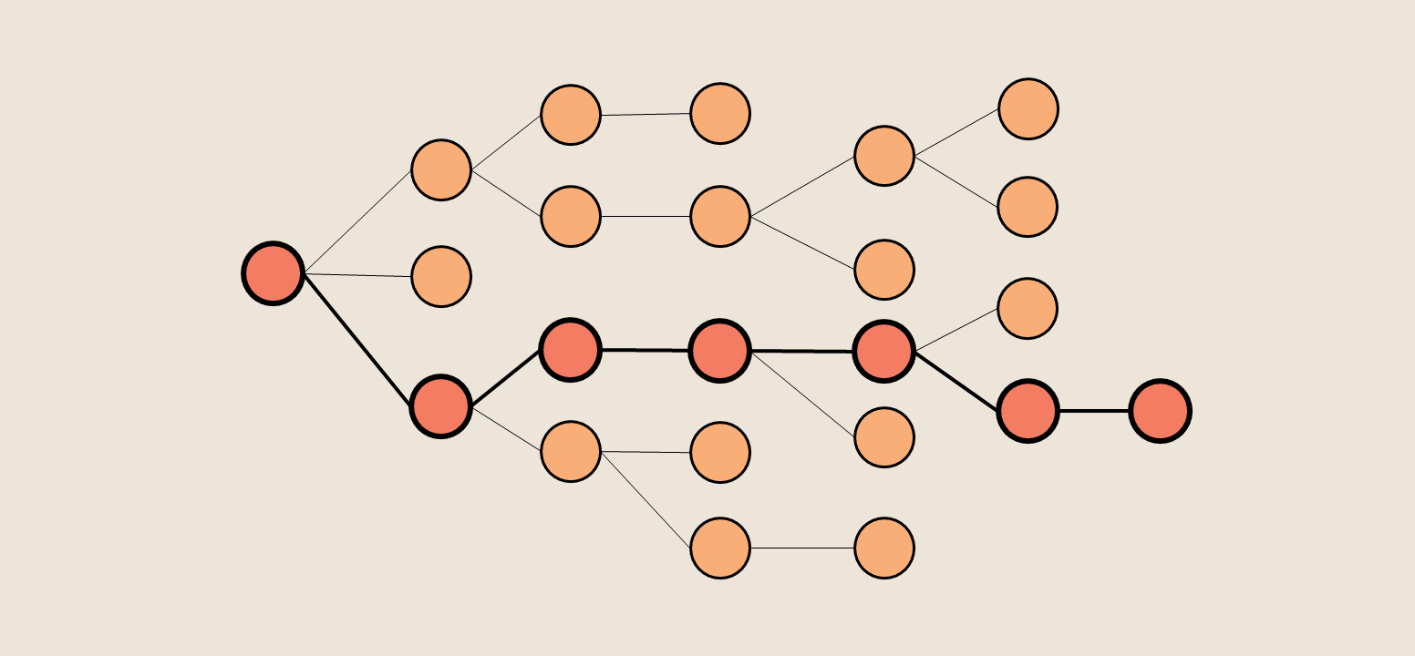
For those unfamiliar, a Monte Carlo tree search algorithm uses random sampling to choose the most promising action, given a high degree of uncertainty. It has often been implemented for game strategy (notably to play the game Go).
In practice, the algorithm looks like:
- Computer is presented with a situation and asked for a decision
- Computer runs “background runs” - games starting from this situation, where every decision is made completely randomly
- Each background run’s final performance is scored
- The runs are grouped by initial move, and performance is averaged
- Computer performs the initial move with highest expected final performance, and repeats 1-5
In our case, playing 2048, the computer would be presented with a layout. It will execute a series of “background runs”. Some, by chance, will be very good games with high final scores, and others will quickly end with low final scores. All of these “background runs” will be grouped by initial move (swipe up, left, down, or right), and the computer then swipes in that direction, hopefully moving incrementally towards the highest expected final score.
Implementation
I previously detailed my implementation of the game logic itself in numpy in the first post in this series, and will rely heavily on the GameLayout class described therein, which holds a game state, including layout & current score, and also provides functionality to update those when a direction is chosen (see GameLayout.swipe(...)).
Setting up
All we need to do to start a game is initialize this class. To make this repeatable, I’m also going to use a random seed.
import numpy as np
np.random.seed(1)
from game import GameLayout

game = GameLayout()
The game is initialized with only 2 nonzero tiles, and I’d prefer to demonstrate with more going on, so let’s generate a random layout that represents a state from a little later in the game, when moves are starting to matter move. To do this, I’ll leverage the GameLayout.swipe(...) functionality with 40 random moves.
for dummy_move in np.random.choice(['w','a','s','d'], size=40):
    try:
        game.swipe(dummy_move)
    except:
        print("Random move was invalid.")
        continue
Now, if you look at game.layout, it should look like:
[ 4,  4,  0,  0,
  2, 16,  0,  0,
  4, 32,  4,  0,
  2, 16,  8,  0]
Simulating outcomes
Next, let’s go to Monte Carlo! All functionality discussed here is contained in my MonteCarloGameDriver class, but I’ll go through it step by step first.
First, we want to make a copy of the game. It’s important to make a “deep copy”, which will actually duplicate the elements inside the game object. Otherwise, when we swipe on the copy it will update the original game.layout too!
from copy import deepcopy

game_copy = deepcopy(game)
game_copy.reset() # removes prior moves/layouts
Now, we will completely randomly run this copy game. This will look very like the GameDriver class discussed in my previous post here.
while game_copy.active:
    moves = ['w','a','s','d']
    np.random.shuffle(moves)
    for move in moves:
        try:
            game_copy.swipe(move)
            break
        except:
            # move didn't work, try next move
            continue
After this snippet runs, we have a finished copy game, including a final score and all moves performed/layouts seen. In fact, we can look at game_copy.final_layout and see how far the game got:
[  4,   2,  16,   4,
 256,  16,   4,   8,
   4,  32,  64,   2,
   2,   8,  16,   4]
This random game achieved a maximum tile of 256, and we can also see that its final score (stored in game_copy.score) was 2,344.
What’s most important to note is this: the initial move this random simulation took (stored as game_copy.moves[0]) was to swipe up.
Choosing optimal action
So should the computer, then, swipe up? A single simulation doesn’t have any differentiating power. Instead, we should repeat this procedure several times and take the average score for each initial move.
This procedure is implemented in my MonteCarloGameDriver.simulate(game, simulation_size) method, which takes a game and runs simulation_size number of random games starting from that initial gamestate.
Let’s see what happens when we use .simulate(...) on our random game described earlier. As a reminder, the layout was:
[ 4,  4,  0,  0,
  2, 16,  0,  0,
  4, 32,  4,  0,
  2, 16,  8,  0]
Let’s import the MonteCarloGameDriver class and run 20 simulations.
from simulator import MonteCarloGameDriver

driver = MonteCarloGameDriver()

driver.simulate(game, 20)
The output of this is game_performance, a dictionary mapping each move - ['w','a','s','d'] - to the average score that first move produced during the simulations. In this case, we get:
game_performance = {'w': 1101.6, 'd': 1038.6666666666667, 'a': 669.0}
Now, we can say that the computer should swipe up, w, as this initial move has the highest expected score, given our simulations.
Performance
Now we’ve covered what the algorithm does and how to implement it, let’s see how it actually does!
Benchmarking
First, lets establish a metric of success.
A low bar would be for the computer to perform consistently better than random, but hopefully we can expect that.
A medium bar would be for the computer to achieve 2048 the majority of the time.
A more personal goal of mine would be to have the computer beat me - or rather, to best my own personal highest-scoring game, which achieved 34,828.
Results
Using the Monte Carlo method I ran 10 sample games for each simulation size - [5, 20, 50, 100, 150]. For comparison, I also ran 10 completely random games to see how much improvement we get with running simulations.
Plotted below, you can see the final scores (after the entire game), by simulation size.
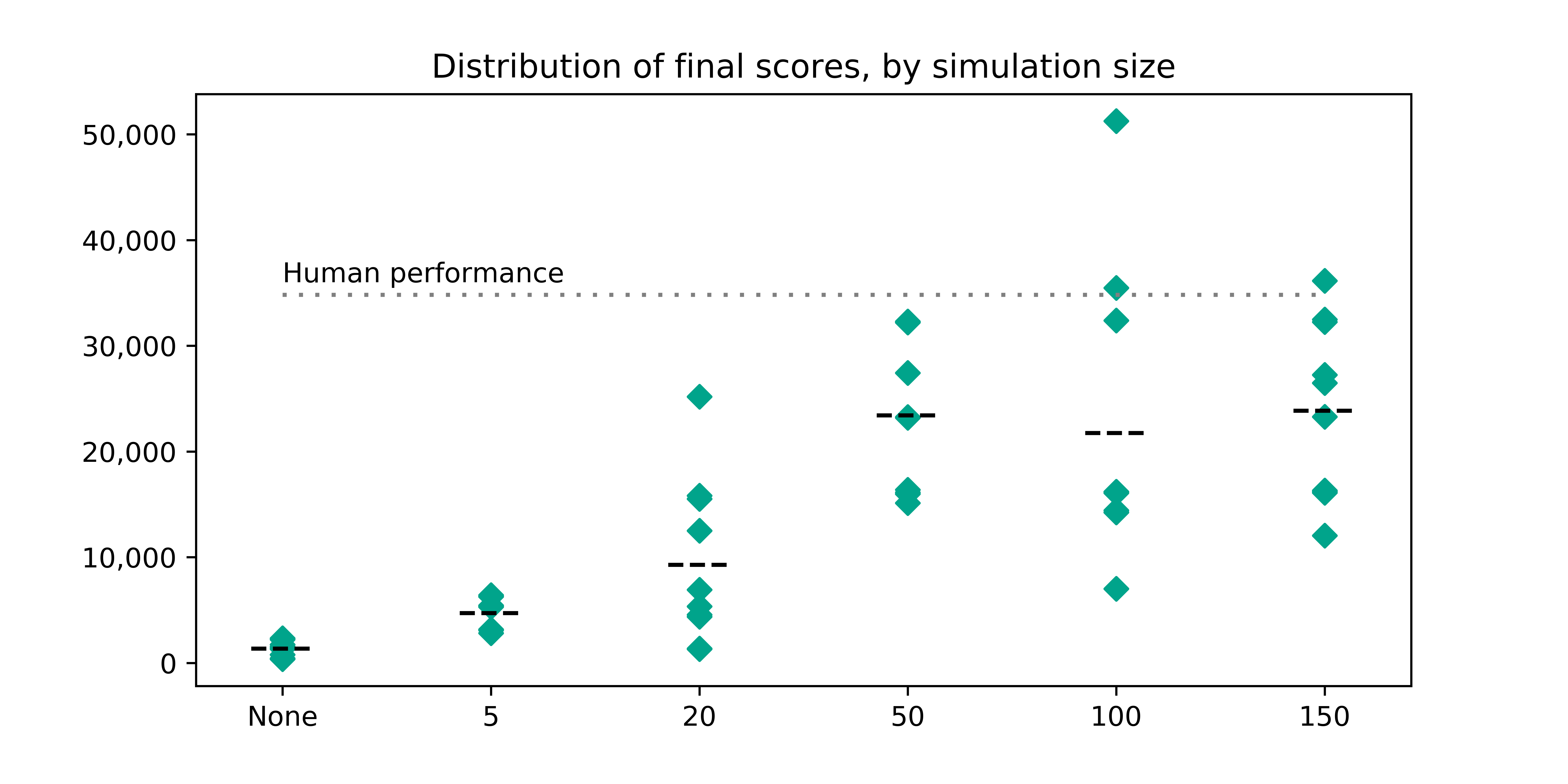
We can see that the huge performance gain happens somewhere between running 20 and 50 background runs at each step. Interestingly, there isn’t dramatic improvement in average score (denoted by the horizontal lines) with additional simulations after 50 - however, we can see that the variance increases, pushing a whopping 3 games above my own personal best!
Also impressively, we can see the maximum tile each game achieves move upward as simulation size increases.
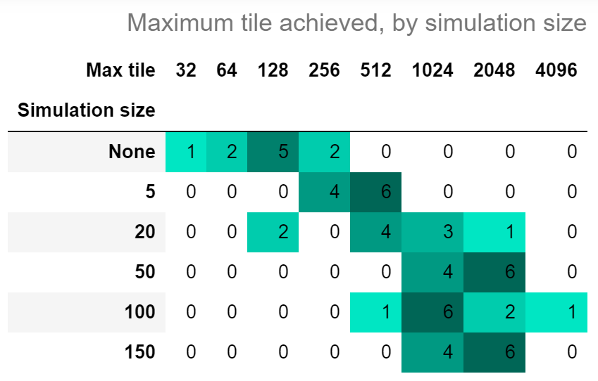
I will declare this approach a success - with just 50 background runs at each step, the computer was able to achieve the 2048 tile 60% of the time, and the 1024 tile the remaining 40%.
Code
Complete code can be found in my 2048 git repository.
This section of the project relies on numpy and pytorch 1.1.0. Additional packages (such as widgets and matploblib) may be required to run any notebooks in the repository.